How Vector Databases Search: A Practical Guide to IVF, HNSW, PQ & ScaNN

Introduction

Most modern applications, from image similarity to RAG systems, depend on fast vector search. Once you embed text, audio, or images into high-dimensional vectors, finding the closest matches turns into an approximate nearest neighbor problem, and that's where vector databases like FAISS, Milvus, Pinecone, Weaviate, and Elasticsearch come in.

Under the hood, though, these systems use very different indexing strategies. Some cluster the data (IVF), some build a graph (HNSW), some compress aggressively (PQ), and some lean on learned heuristics tuned for speed (ScaNN).

This post breaks down how each of these indexes works, why it exists, and how to pick the right one, using plain examples instead of academic notation, and drawing on what we've learned running Hoomanely's own RAG and retrieval systems.

Why vector indexes matter

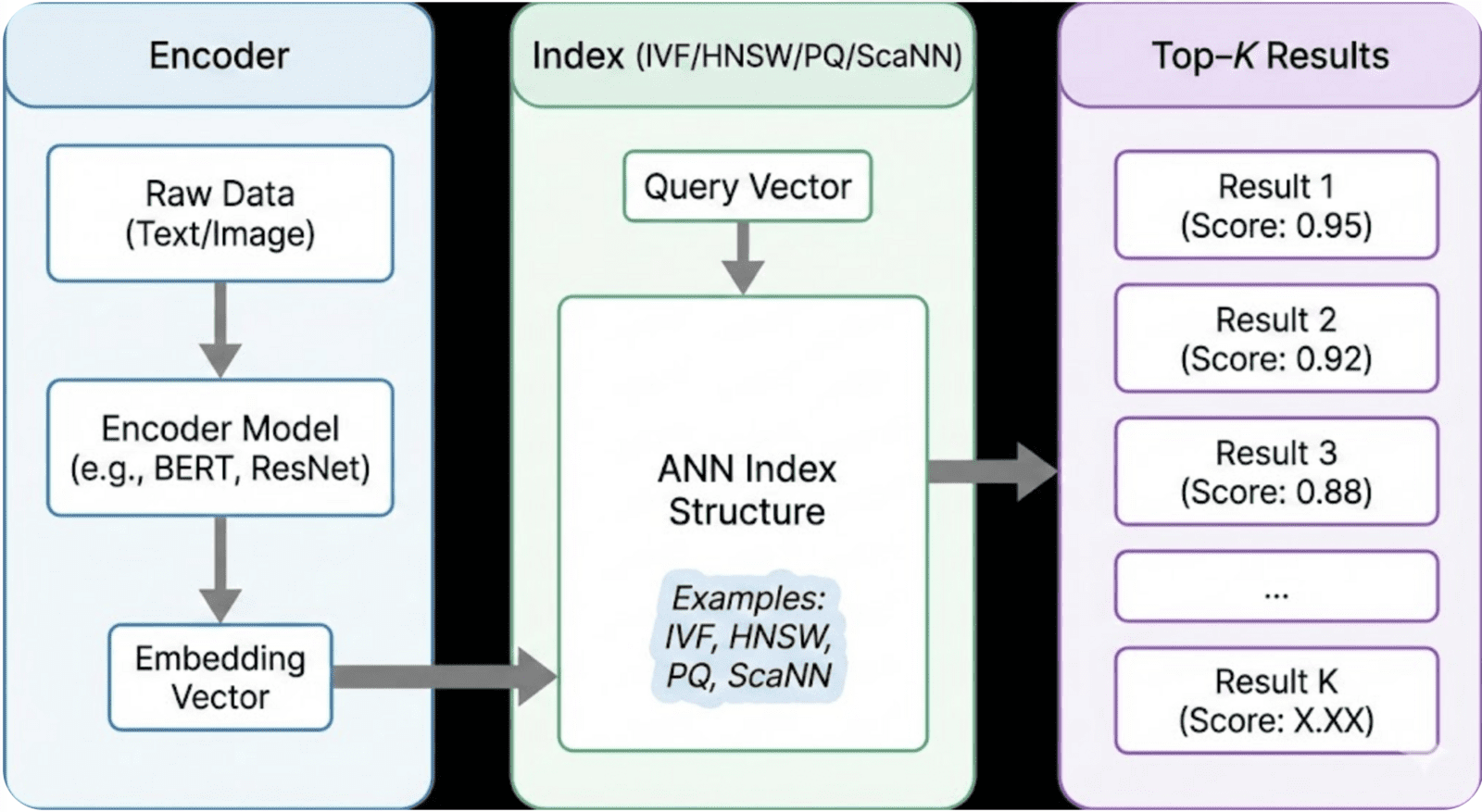
A naive vector search checks every embedding, which is O(N). That's fine for a million vectors and a serious problem at a hundred million. ANN indexes speed things up by cutting the search space (IVF), navigating only the promising parts of it (HNSW), compressing vectors to fit in RAM (PQ), or pruning compute with learned heuristics (ScaNN). At Hoomanely, where a single query can touch thousands of pages across hundreds of veterinary PDFs, low-latency retrieval isn't optional, it's what keeps the product usable.

IVF, the inverted file index

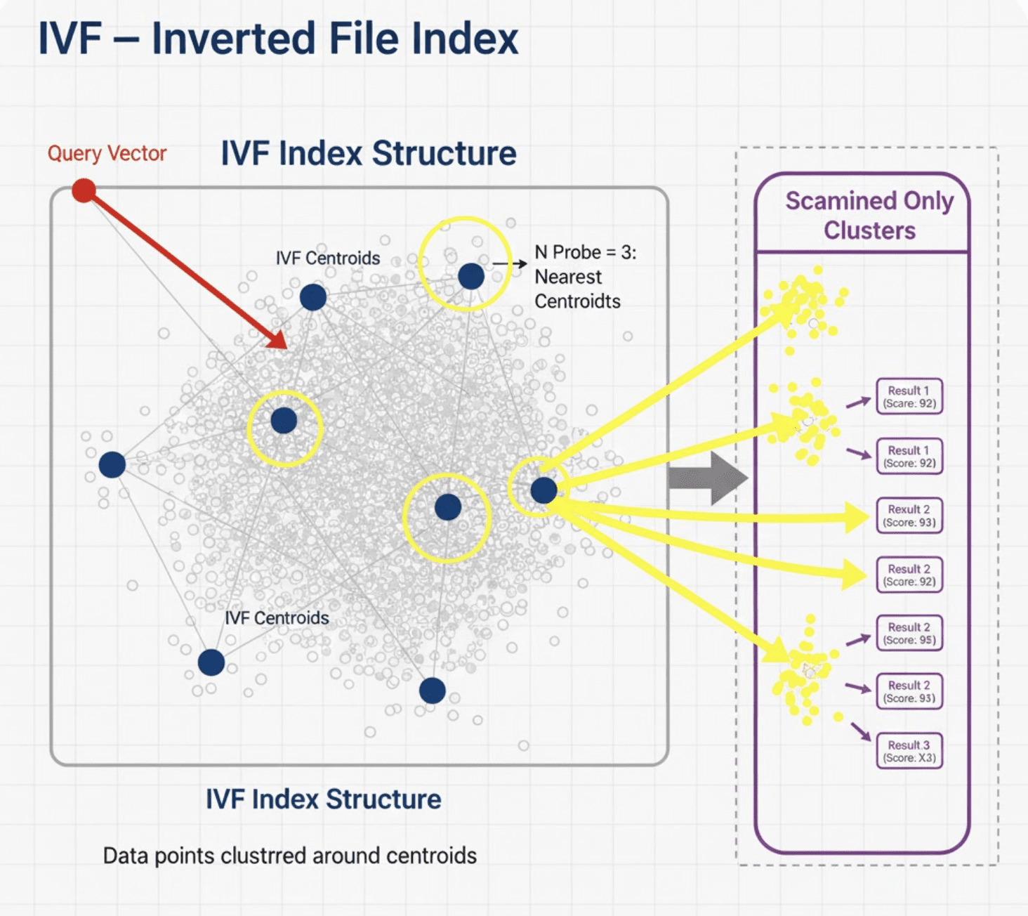
IVF partitions the vector space using clustering, usually k-means, so a search only touches a handful of clusters instead of everything. Think of a library where the shelves are numbered first, and a search only walks to a few of them.

How it works: run k-means to get nlist centroids, assign every vector to its nearest centroid, then at query time assign the query to the nearest centroids and search only inside those partitions. With 1,024 clusters and 8 probed per search, that's a 128x reduction in search cost.

Pros: memory-efficient, easy to scale, pairs well with PQ (IVF-PQ). Cons: quality depends heavily on the clustering, and it's not a great fit for oddly shaped data distributions.

HNSW, the hierarchical graph index

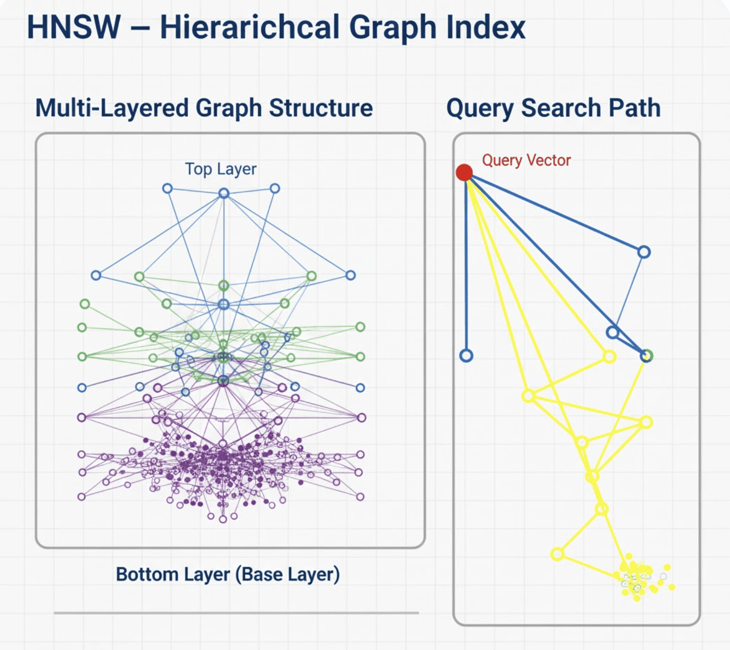
HNSW builds a multi-level navigable graph where each node links to its nearest neighbors. Higher levels give long jumps across the space, lower levels give precision. It's a bit like Google Maps with highways on the top layer and local roads underneath.

How it works: build several layers, with fewer nodes at each higher layer, insert each vector at a random layer height, then search by starting at the top layer, moving greedily toward the query, dropping down a layer at a time, and finally exploring neighbors at ground level to return the top matches.

Pros: the highest recall at low latency among these options, handles real-time inserts and deletes well, and skips expensive clustering entirely. Cons: a larger memory footprint, and slower to build on large datasets. Pinecone, Milvus, Weaviate, and FAISS all offer HNSW.

PQ, product quantization

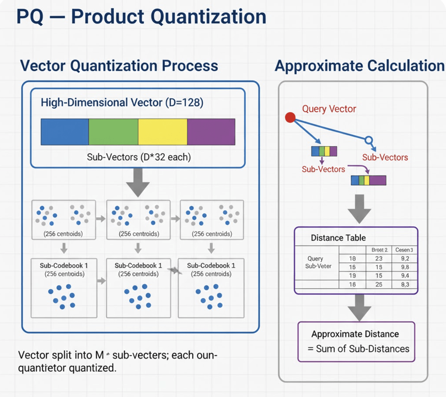
PQ compresses each vector into small discrete codes, trading some accuracy for a large reduction in memory. Picture splitting a 768-dimensional vector into 16 chunks of 48 dimensions each, then encoding every chunk against a small lookup table.

How it works: split each vector into m sub-vectors, cluster each subspace on its own, store only the cluster IDs, then at search time precompute distances to all the codebooks and estimate distances quickly from there.

Pros: shrinks vectors by 8x to 32x, lets massive datasets fit in RAM, and pairs well with IVF as IVF-PQ. Cons: lower recall than HNSW, and codebook training needs care. FAISS-PQ and Milvus's IVF-PQ both use this approach.

ScaNN, Google's high-performance ANN

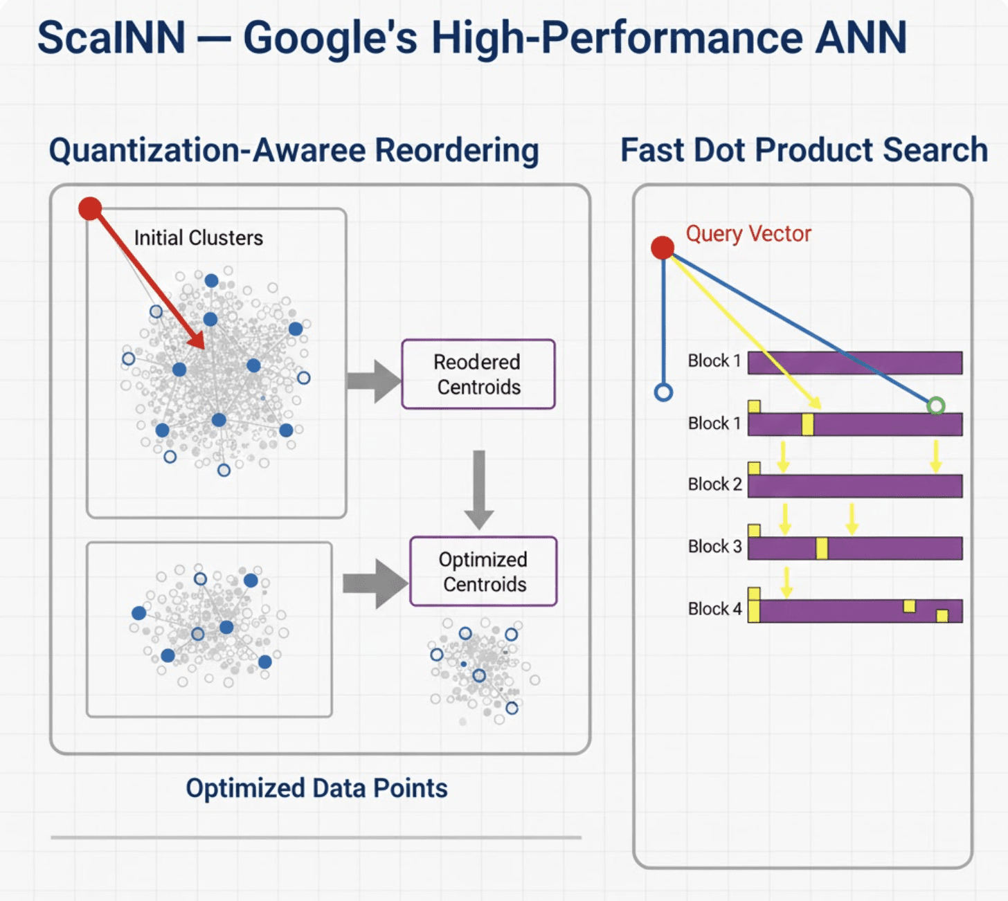
ScaNN combines tree-based partitioning, anisotropic quantization, and learned pruning, and its main strength is balancing speed and accuracy without burning through memory.

In practice it uses tree-like IVF partitioning to narrow the search, quantized scoring for faster distance math, and residual reordering to rescore the top candidates exactly. That combination runs fast on both TPUs and CPUs.

Pros: high recall at moderate memory cost, strong with text embeddings, and performs well in batch mode. Cons: harder to tune than the alternatives, and less common in production than HNSW. Google Search and Vertex Matching Engine both run on it.

Comparing all four

How we apply this at Hoomanely

Our veterinary RAG pipeline has to pull the right pages out of thousands of medical documents, which meant testing IVF, HNSW, and PQ combinations directly against our own data. HNSW gave us the strongest recall, especially on long clinical queries. IVF-PQ gave us the smallest memory footprint, which matters with large document sets. A hybrid IVF-HNSW setup gave us fast retrieval even in CPU-only environments. Picking the right index is a direct lever on how fast and how accurate our answers are.

Takeaways

• IVF is a solid first choice for scalable, static datasets.
• HNSW is the strongest all-rounder when you need high recall and frequent inserts.
• PQ earns its place when memory is tight or the dataset is huge.
• ScaNN suits high-speed text retrieval, particularly in cloud environments.
• The right index depends on your constraints: memory, latency, recall, and how often the vectors change.