IMU Calibration and Drift Management in Consumer Trackers

Have you ever wondered how your pet's GPS tracker knows whether they're running, resting, or digging in the backyard? Or why sometimes the tracker seems to lose accuracy after a few weeks of use? The secret lies in a sophisticated component called an Inertial Measurement Unit, a sensor that measures motion across nine degrees of freedom.

This post explores the engineering challenges of IMU calibration using our EverSense pet tracker as a real-world case study. Think of IMU calibration like tuning a high-precision instrument, even the best sensors need regular adjustment to maintain their accuracy. Just as atomic clocks require environmental compensation, IMU sensors experience drift that compounds over time, affecting everything from activity classification to dead reckoning navigation.

The tracker uses the ICM-20948, a 9-axis IMU combining a 3-axis accelerometer, 3-axis gyroscope, and 3-axis magnetometer. This sensor fusion architecture enables sophisticated motion analysis, but it also introduces complex calibration challenges spanning mechanical, electromagnetic, and thermal domains.

The problem: multi-domain error sources in 9-axis IMUs

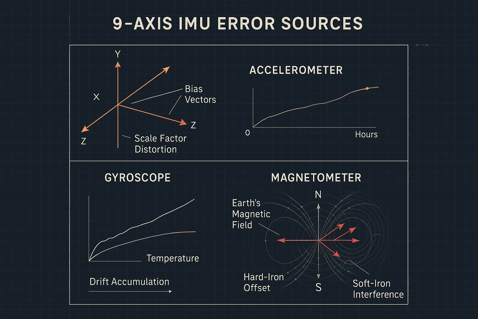
The ICM-20948's 9-axis architecture provides rich motion data, but each sensor type exhibits unique error characteristics that interact in non-obvious ways.

For the accelerometer, static bias and scale factor errors show up as a zero-g offset, bias present even in zero acceleration conditions, typically plus or minus 50-100mg between units; a scale factor error where sensitivity deviates from the nominal 1g per LSB, usually 0.5-3%; cross-axis sensitivity, where acceleration along one axis creates false readings on perpendicular axes due to mechanical misalignment; and nonlinearity, where response deviates from linear at high accelerations above 4g. For pet tracking, accelerometer accuracy directly impacts activity classification, a 50mg bias error translates to roughly 5% error in activity intensity estimation, enough to misclassify walking as running or miss subtle behavior changes indicating health issues.

The gyroscope has the drift problem. It measures angular velocity around each axis and is exceptional for tracking rapid orientation changes, but suffers from integration drift, small errors compounding exponentially over time. The ICM-20948 specifies 0.015 degrees per second per root Hz white noise, manifesting as angle random walk of roughly 0.15 degrees per root hour. Bias instability drifts even when stationary, typically 0.1-0.5 degrees per second for consumer-grade MEMS gyros. Temperature-induced drift is around 0.03 degrees per second per degree C, a 30 degree C temperature swing, common when a pet moves from indoors to summer sun, introduces 0.9 degrees per second of additional bias. Integrate a 0.2 degree per second gyroscope bias error over one hour and you accumulate 720 degrees of heading uncertainty, which is why gyroscopes alone can't maintain long-term orientation, they need continuous correction from complementary sensors.

The magnetometer faces hard-iron, soft-iron, and temporal interference. It measures Earth's magnetic field, roughly 25-65 microtesla depending on location, to determine absolute heading, theoretically elegant but practically challenging in electronic devices. Hard-iron distortion comes from ferromagnetic materials creating constant offset fields, the tracker's Li-ion battery steel can, PCB mounting hardware, and speaker magnets contribute 10-30 microtesla of constant bias. Soft-iron distortion comes from ferrous materials distorting Earth's field non-uniformly depending on device orientation, requiring full 3x3 correction matrices. Temporal interference comes from the ESP32-S3's Wi-Fi transmitter, up to 20dBm at 2.4GHz, and the RFM95W LoRa radio, 14dBm at 915MHz, generating dynamic electromagnetic fields pulsing with transmission bursts. The engineering challenge: distinguishing Earth's 50 microtesla field from a 30 microtesla constant offset plus 5-10 microtesla dynamic interference from radios located just 15mm away on a compact PCB, requiring both static calibration via ellipsoid fitting and dynamic rejection via temporal filtering during known transmission windows.

Approach: three-tier calibration architecture

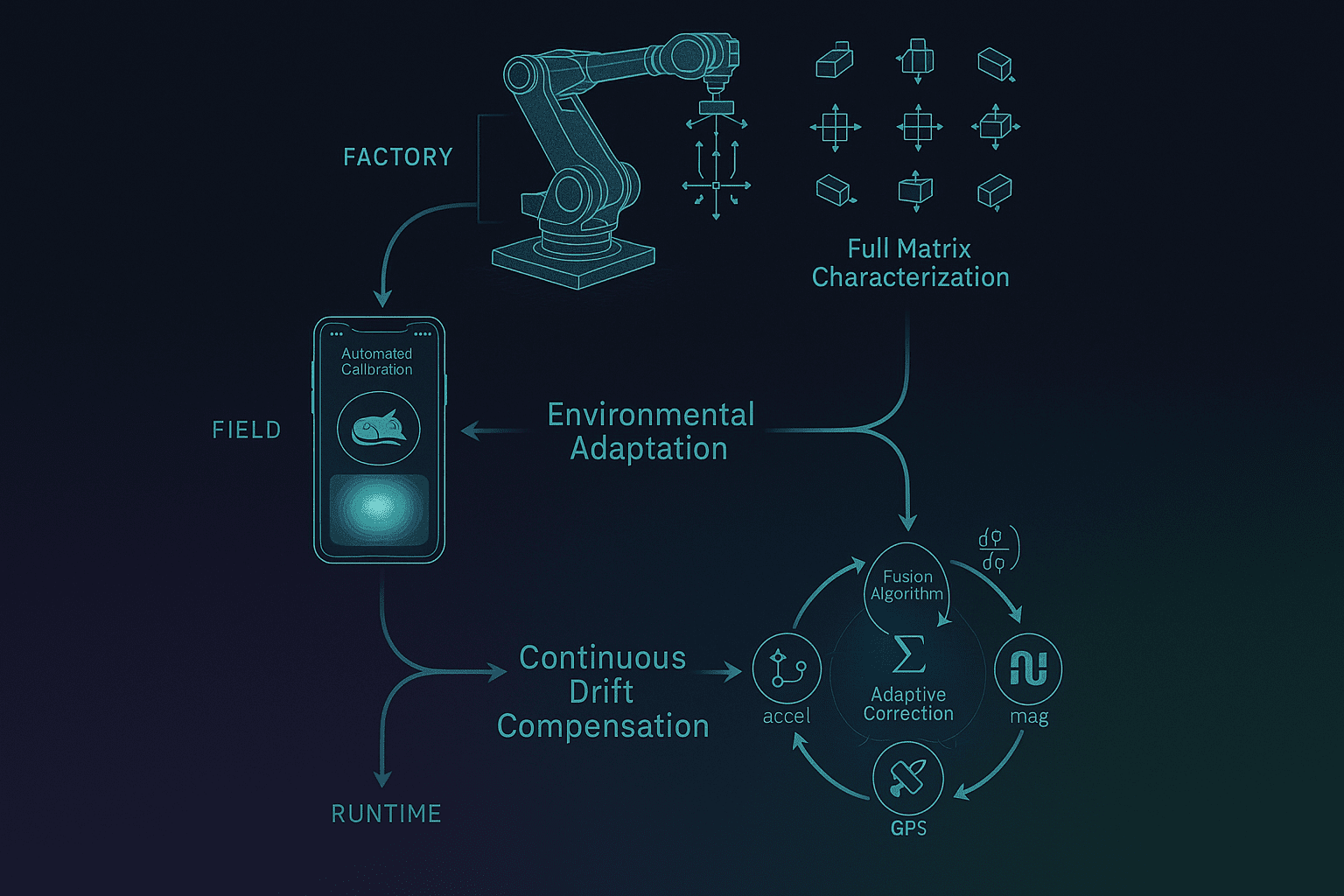
Rather than treating calibration as a one-time factory process, we've architected a hierarchical system addressing error sources at different time scales and operational contexts.

Factory calibration handles systematic error characterization. During production, each device undergoes parametric testing on a precision 6-DOF motion platform. The key insight: we're not just measuring current offsets, we're characterizing the transfer function of each sensor axis, including full 3x3 scale and cross-axis compensation matrices, temperature-dependent polynomial coefficients for gyroscope bias measured at -10, 25, 45, and 60 degrees C, magnetometer ellipsoid parameters in a controlled low-EMI environment, and sensor timing calibration accounting for group delay differences between accelerometer, gyroscope, and magnetometer sampling. This comprehensive characterization captures 70-80% of systematic errors and establishes a device-specific baseline stored in the W25Q512JV flash's protected calibration sector.

Field calibration handles installation and environmental adaptation. Factory calibration occurs in a controlled environment, but field deployment introduces new error sources, mounting stress where the PCB flexes slightly when mounted in the collar enclosure, shifting accelerometer bias by 20-40mg, local magnetic anomalies where ferrous objects in the pet's environment create local distortions, and installation-specific hard-iron from the exact positioning of battery, antenna, and PCB creating unique magnetic signatures per assembly. Field calibration adapts the factory baseline to these installation-specific factors through automated data collection during normal device usage.

Runtime correction handles adaptive drift compensation. Even with excellent static calibration, sensors drift during operation due to temperature cycling, thermal hysteresis in MEMS structures, component aging, stress relaxation in suspension springs, and temporal electromagnetic interference from Wi-Fi and LoRa transmission bursts. Runtime algorithms continuously monitor sensor consistency, detect anomalies, and apply dynamic corrections without requiring user intervention. This layer is where the most sophisticated engineering happens, balancing computational cost, power consumption, and correction accuracy in a resource-constrained embedded system.

Factory calibration: beyond simple offset correction

The naive approach to accelerometer calibration measures each axis pointing up and down relative to gravity, computing a simple offset and scale factor. Instead we perform 12-position testing that fully characterizes the 3x3 transformation matrix:

// Full 3×3 calibration matrix approach
typedef struct {
    float scale_matrix[3][3];  // Accounts for scale + cross-axis
    float offset[3];            // Zero-g bias
    float noise_floor[3];       // Per-axis noise characterization
} accel_calibration_t;
 
// Apply calibration transformation
void calibrate_accel(float raw[3], float calibrated[3],
                     const accel_calibration_t *cal) {
    // Remove offset
    float temp[3];
    for (int i = 0; i < 3; i++) {
        temp[i] = raw[i] - cal->offset[i];
    }
  
    // Apply scale and cross-axis correction matrix
    for (int i = 0; i < 3; i++) {
        calibrated[i] = 0;
        for (int j = 0; j < 3; j++) {
            calibrated[i] += cal->scale_matrix[i][j] * temp[j];
        }
    }
}

This matrix-based approach corrects not just scale factors but also the 1-3% cross-axis sensitivity simple calibration ignores. The result: accelerometer orthogonality error drops from 2-3 degrees to under 0.5 degrees.

For gyroscope temperature compensation we've implemented a second-order polynomial model rather than simple linear correction: Bias(T) equals b0 plus b1 times delta-T plus b2 times delta-T squared.

Field calibration: exploiting natural pet behavior

The engineering challenge with pet trackers is that we can't ask users to precisely orient the device. Instead we've designed algorithms that opportunistically collect calibration data during normal usage.

Magnetometer ellipsoid fitting is where the engineering gets particularly interesting. Hard-iron and soft-iron distortions transform the ideal sphere of magnetic field measurements into an ellipsoid offset from the origin. We collect magnetometer samples during periods of active motion, when gyroscope magnitude exceeds 10 degrees per second, to ensure diverse orientations. The algorithm fits a 3D ellipsoid to this point cloud, where the center represents hard-iron offset and the radii ratios characterize soft-iron distortion. We've implemented a recursive least-squares approach updating ellipsoid parameters with each new sample, converging to under 5% error after 200-300 samples, roughly 10 minutes of normal pet activity.

Runtime correction: complementary filter design

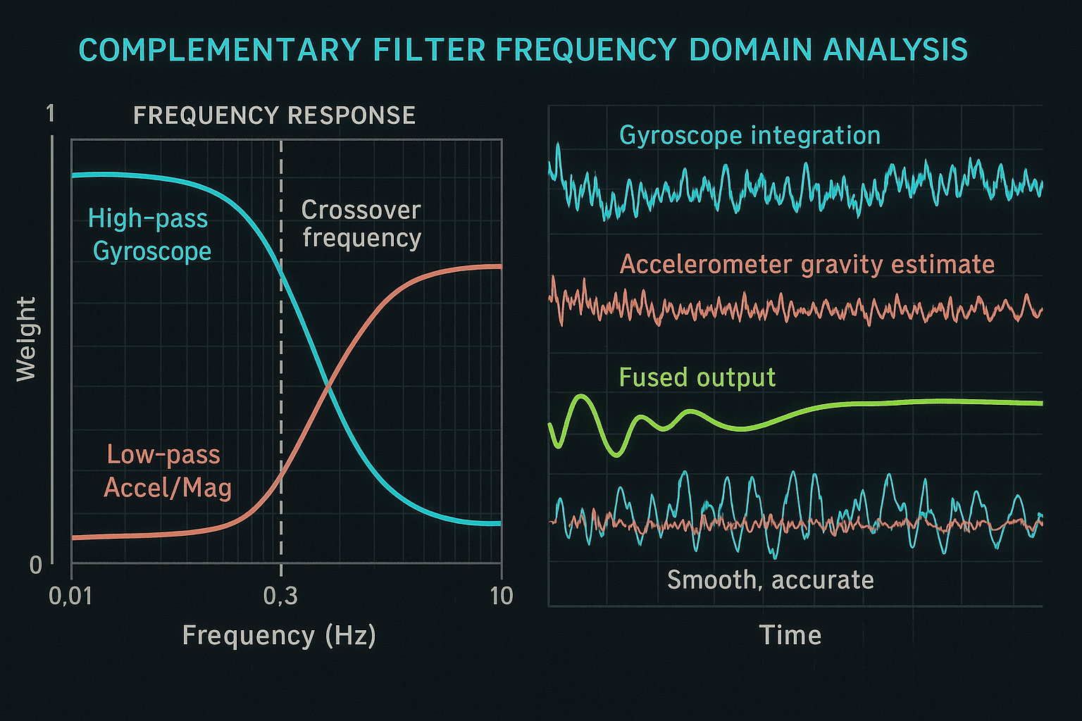
This is where the 9-axis architecture truly shines. Each sensor type has complementary strengths and weaknesses. The gyroscope offers high-frequency accuracy but suffers low-frequency drift, with fast 100Hz bandwidth. The accelerometer offers a gravity reference but suffers motion noise, filtered to about 1Hz. The magnetometer offers absolute heading but suffers EMI sensitivity, also filtered to about 1Hz. GPS offers absolute position and heading but suffers latency and dropouts, at a very slow 1Hz.

We implement a complementary filter fusing these sources with frequency-dependent weighting:

// Simplified complementary filter core
void update_orientation(float dt) {
    const float ALPHA = 0.98f;  // Trust high-freq gyro, low-freq accel/mag
  
    // High-pass: integrate gyroscope (fast dynamics)
    orientation[ROLL]  += gyro[X] * dt;
    orientation[PITCH] += gyro[Y] * dt;
    orientation[YAW]   += gyro[Z] * dt;
  
    // Low-pass: gravity reference from accelerometer
    float accel_roll  = atan2f(accel[Y], accel[Z]);
    float accel_pitch = atan2f(-accel[X],
                        sqrtf(accel[Y]*accel[Y] + accel[Z]*accel[Z]));
  
    // Fuse with complementary weights
    orientation[ROLL]  = ALPHA * orientation[ROLL]  + (1-ALPHA) * accel_roll;
    orientation[PITCH] = ALPHA * orientation[PITCH] + (1-ALPHA) * accel_pitch;
  
    // Magnetometer provides absolute yaw (heading)
    if (mag_valid && gps_speed < 0.5) {  // Only trust mag when stationary
        float mag_yaw = calculate_tilt_compensated_heading();
        orientation[YAW] = ALPHA * orientation[YAW] + (1-ALPHA) * mag_yaw;
    } else if (gps_valid && gps_speed > 2.0) {  // Use GPS heading when moving
        orientation[YAW] = ALPHA * orientation[YAW] + (1-ALPHA) * gps_heading;
    }
}

The key engineering detail: the complementary filter coefficient of 0.98 determines the crossover frequency. At a 100Hz sample rate this yields roughly a 0.3Hz crossover, meaning the gyroscope dominates above 0.3Hz for fast motions, while accelerometer and magnetometer dominate below 0.3Hz for slow drifts.

Key takeaways for engineering teams

Calibration is a control systems problem, not a one-time measurement. Effective IMU calibration requires feedback loops operating at multiple time scales, fast runtime correction at 10-100Hz, medium-term environmental adaptation over hours to days, and slow predictive maintenance over weeks to months. Design your architecture to support all three layers from day one.

MEMS sensors exhibit non-ideal behavior simple calibration misses. Cross-axis sensitivity, nonlinearity, and temperature hysteresis are real effects that compound in production, budget engineering time for full matrix characterization and polynomial temperature models, the 15% accuracy improvement is worth the extra complexity.

Electromagnetic compatibility is critical in integrated IoT devices. When your IMU shares a PCB with multiple radios, EMI mitigation must be baked into both hardware layout and firmware algorithms, temporal blanking and outlier rejection aren't optional, they're essential for reliable magnetometer operation.

Sensor fusion transforms noisy measurements into reliable information. No single sensor maintains accuracy across all conditions, complementary filtering with adaptive coefficients lets you extract the best performance from each sensor while rejecting individual failure modes. The mathematics is straightforward, the engineering lies in tuning crossover frequencies for your specific application.

Fleet-level analytics enable predictive quality. Traditional embedded systems operate in isolation, modern IoT devices can leverage cloud analytics to detect degradation patterns, correlate failures across batches, and trigger proactive interventions, transforming calibration from reactive troubleshooting into predictive maintenance.

And design calibration UX for your actual users. Engineers instinctively design complex multi-step calibration procedures, real users won't complete them, invest in automatic background calibration that leverages natural device usage.

At Hoomanely, we're building intelligent monitoring solutions that enhance pet safety, health, and well-being. The tracker represents our engineering philosophy: sophisticated technology should work invisibly, reliably, and continuously without demanding user attention. The calibration architecture described here ensures trackers maintain exceptional accuracy throughout their lifecycle, whether detecting subtle gait changes that indicate joint problems, distinguishing normal activity from distress behaviors, or providing reliable location tracking during critical moments.