Software

Stable BLE Sensor Streams: MTU, Connection Interval, and End-to-End Buffer Control

Pravin Kumar

02 Feb 2026 — 10 min read

Stable BLE streaming can feel like magic when it works: sensors stay responsive, data arrives smoothly, and the app feels “live” without burning the battery or stuttering the UI. The good news is that this isn’t luck—it’s engineering. When you treat BLE as an end-to-end streaming pipeline (not just a radio link), you can make throughput steady, latency predictable, and jitter boring across different phones, OS versions, and real-world usage.

We’ll start from a target sensor rate and turn it into a measurable throughput + jitter budget, then tune MTU and payload framing to reduce overhead, choose connection interval / latency settings that shape delivery into a stable cadence, and add buffer control so queues never silently grow into lag. We’ll also make sure the Flutter side—decoding, isolates, and UI update frequency—stays fast enough that the app never becomes the hidden bottleneck. The end result is a BLE stream you can trust in production: smooth, repeatable, and easy to validate.

Problem: Why BLE Streams Get “Bursty” in Production

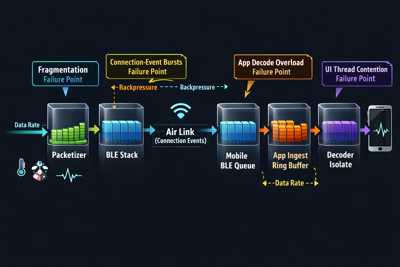
Even if your raw link throughput is “enough,” stability fails when timing mismatches stack up across layers:

Peripheral sends in bursts (scheduler tick, sensor batching, RTOS timing).
BLE link delivers in connection events, not continuously.
Mobile stacks buffer aggressively, then release data to the app in lumps.
Flutter decoding competes with UI, and heavy parsing can starve reads.
UI refresh cadence (and animations) creates periodic CPU pressure.
No backpressure policy means queues grow invisibly until you drop.

A stable stream is not “max throughput.” It’s controlled throughput with bounded jitter and bounded memory growth.

Approach: Engineer to a Budget, Not to a Guess

When BLE streaming feels unstable, the usual instinct is to tweak a couple of knobs—raise MTU, lower connection interval—and hope the stream “locks in.” That can work in a lab, but it’s fragile in production because you’re optimizing one layer without defining what the system is actually trying to guarantee.

A better approach is to treat streaming like any other production pipeline: you define an explicit delivery budget, then you tune each layer to meet it with margin. The budget is what makes tuning measurable, repeatable, and portable across devices.

Convert your sensor target into a throughput + jitter budget

Your sensor target isn’t just “bytes per second.” It’s a quality-of-delivery contract, Start with the non-negotiables you must deliver:

Sample size (bytes/sample)
The actual payload per logical sensor unit, including what the app truly needs (not what’s convenient to emit).
Sample rate (samples/sec)
The stream’s “truth clock.” Even if you batch, this is the rate the consumer experiences.
Acceptable end-to-end latency (ms)
The maximum age of data when it becomes visible/usable (UI, logging, control loop, inference).
Acceptable jitter (P95/P99)
Not the average arrival rate, but how uneven delivery is allowed to be at the tail.

From these, define three explicit budgets:

Useful Throughput Budget

This is the payload your application needs to remain correct and responsive in steady state. Useful throughput is what survives all framing and protocol overhead—it’s the true “sensor value bandwidth.”

What matters here:

Your stream must sustain the useful rate continuously, not just in bursts.
Useful throughput should be measured both:
- At ingress (right after the BLE callback), and
- After decode (because decoding failures/slowdowns effectively reduce throughput).

Jitter Budget

Jitter is the shape of delivery. You can have correct average throughput and still get an unusable stream if delivery is lumpy—because lumpiness causes buffer growth, delayed UI updates, and unpredictable control behavior.

Define jitter in terms of:

Inter-frame arrival variability at the app boundary (not the radio)
Tail jitter (P95/P99), because worst-case burstiness is what breaks UX stability
Burst tolerance, i.e., how much the system can absorb without backlog

End-to-End Latency Budget

This is the “freshness contract.” Latency is not only BLE; it’s everything:

time spent waiting for the next connection event
time sitting in OS queues
time waiting for decode scheduling
time waiting for UI cadence

Latency should be measured as:

Sensor time → usable time (not “notification received”)
P50 and P95/P99, because tail latency is where streams feel broken

Once you define the useful throughput and jitter budgets, you need to account for the fact that BLE does not deliver “useful bytes.” It delivers packets with overheads and constraints that vary by device, OS, and runtime conditions.

Instead of guessing, explicitly name each overhead source so you can reason about where the bandwidth and stability actually go:

Framing overhead

This includes everything you add for correctness and evolvability:

sequence numbers
timestamps
message type/version
checksum/CRC (if used)

Framing overhead is not “waste”—it’s what makes the stream debuggable and stable under loss/reorder. But you still want it to be predictable and amortized (i.e., don’t pay heavy per-sample overhead if your stream is high-rate).

ATT / GATT overhead

This is where “set MTU higher” can help, but only if your framing plays along.

ATT/GATT introduces:

per-attribute operation overhead
notification/indication semantics
fragmentation risk if payload framing doesn’t align with negotiated MTU

The key stability point: fragmentation doesn’t just reduce throughput—it increases processing cost, increases burstiness, and increases reassembly complexity. Those three are what create jitter and app-side backlog.

BLE Link Layer overhead

The link layer determines what happens during connection events: scheduling, retransmissions, and packetization behavior. Even if your app thinks in “frames,” the link delivers in terms of connection-event opportunities.

This overhead shows up as:

payload vs control traffic ratio
retransmission behavior under interference
burst delivery tied to connection events

The implication for your budget: you should assume your effective throughput and arrival smoothness will degrade in real environments unless you’ve engineered headroom and buffering rules.

Encryption overhead (if enabled)

Encryption can change:

effective payload available per packet
processing time per packet
retry behavior under poor conditions

Mobile stack buffering effects

This is the most common blind spot.

The phone isn’t a passive pipe. It buffers, coalesces, schedules, and sometimes batches delivery to your app depending on:

OS scheduling pressure
background policies
Bluetooth stack decisions
CPU contention from UI or other apps

Sustained throughput with margin

Your goal is not “meet the rate.” It’s “meet the rate with resilience.”
Margin protects you from: interference, device differences, UI contention, periodic OS scheduling effects

Drop rate as a correctness signal

Drops aren’t just data loss—they are a sign your pipeline lacks control. Drops typically mean one of these is true:

sender is producing faster than receiver can ingest or decode
buffering is unbounded and you hit memory/queue limits
fragmentation/reassembly cost exceeds available CPU budget
your app’s “hot path” has hidden work (allocations, copies, parsing)

Even if your use case tolerates some loss, you still want drop rate as a diagnostic metric because it reveals where the system is failing.

Latency (median + tail) as user trust

Median latency tells you normal responsiveness. Tail latency tells you whether the stream feels stable.

A stable stream keeps tail latency bounded over long runs, not just short tests.

Jitter as the hidden UX killer

A stream can have correct throughput and latency averages, but poor jitter will:

force bigger buffers
cause decode spikes
increase UI scheduling pressure
make controls feel inconsistent

If jitter isn’t bounded, your only workaround becomes “increase buffering,” which trades jitter for lag—and lag is what users notice.

Memory growth (queue drift) as the ultimate stability check

Queue drift is the early warning sign that you’ll eventually hit:

delayed UI updates
large GC pauses / allocation pressure
dropped frames
disconnection/reconnect loops

Process: MTU, Connection Interval, and Buffer Control

MTU: Pick it for payload framing

Higher MTU reduces overhead per useful byte if you can fill it efficiently. But MTU only helps when:

your packets are large enough to benefit, and
you avoid fragmentation and partial fills that reintroduce overhead.

Practical framing rule:

Define a frame that contains a batch of samples.
Frame size should be:
- < (MTU - header) for “single-ATT-write” delivery, OR
- a clean multiple that your receiver reassembles cheaply.

A typical stable pattern:

Batch N samples per frame so that frames arrive at a steady cadence, e.g. 20–50 frames/sec.
Keep frame parsing constant-time and predictable.

That’s a nice cadence: not too frequent to cause overhead, not too big to increase burstiness.

Key anti-patterns

“One sample per notification” at high Hz → too much overhead + scheduling jitter.
“Huge frames” that exceed what the phone can decode fast → app becomes bottleneck.
MTU maxed, but frames half empty → you pay overhead anyway.

What to measure

negotiated MTU distribution across devices
average payload fill ratio (%)
frame reassembly CPU time

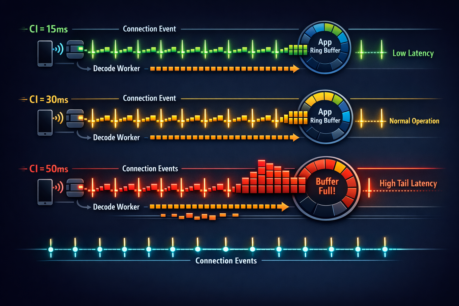
Connection Interval (CI) + Slave Latency: Treat as a shaping tool

BLE delivers data in connection events. CI sets how often those events occur.

Short CI (e.g., 7.5–15 ms): more events, lower latency, higher radio duty
Long CI (e.g., 30–50 ms): fewer events, more bursty, better power

Slave latency allows the peripheral to skip connection events when it has nothing important to send (power saver), but it can also worsen burstiness if used carelessly.

Stability-first guidance

Pick a CI that makes your required throughput achievable without relying on bursts.
Keep slave latency low (or zero) during active streaming, unless you have a clear power reason and a proven buffering model.

This “two-profile” strategy is often what separates a stable product stream from a lab demo.

Peripheral packetization: Make the sender predictable

A stable sender has three properties:

Fixed cadence: frames at consistent intervals (e.g., every 40–60 ms)
Bounded burst size: don’t dump huge bursts after delays
Deterministic framing: receiver can reassemble quickly

Packetization checklist

Use a sequence number per frame (wrap OK).
Add timestamp (sensor-time) to detect lag and jitter correctly.
Add frame type/version to evolve formats safely.
Optional: a tiny CRC per frame if corruption detection matters for your domain.

Golden rule: If you can’t explain your framing on a whiteboard in 60 seconds, your future debugging will be painful.

5) Flutter: Make decoding a separate, metered subsystem

A common failure mode is accidental: decoding on the UI isolate “because it works.” Then a slightly older device, or an animation-heavy screen, causes decode delays and the BLE callback can’t keep up.

Stable Flutter pattern

BLE callback does minimal work: copy bytes into a ring buffer (or chunk queue).
Decoder runs in an isolate (or a dedicated worker) with:
- a fixed max batch size per tick
- time budgeting (“decode up to X ms then yield”)
UI receives downsampled updates (don’t redraw at sensor Hz).

UI cadence rule

If your sensor is 100–500 Hz, UI updates should often be 10–30 Hz.
Let UI show state, not raw samples.

This single decision eliminates a huge class of “mystery jitter.”

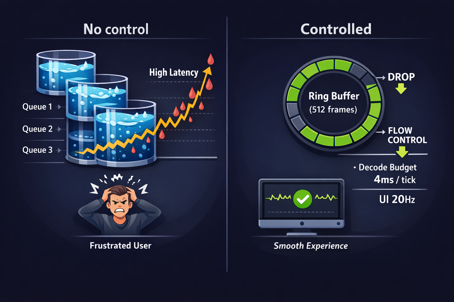
Buffer Control: Prevent Queue Growth by Design

Think of each boundary as a queue:

Peripheral TX queue
Controller/stack queue
OS callback queue
App ingest queue
Decode queue
UI update queue

A stable system has explicit policies at each:

Hard bounds + drop strategy (when allowed)

If your data can tolerate loss (e.g., high-rate IMU for a smoothed UX):

Use a ring buffer with a fixed capacity.
When full: drop oldest (keeps “most recent” fresh), or drop newest (preserves continuity).
Record drops as metrics.

Backpressure signal (when loss is not allowed)

If you must not lose data:

Implement a lightweight flow control:
- peripheral slows frame rate when app lag increases
- app sends “window size” or “ready/not-ready” control over a separate characteristic
Keep it simple: 2–3 states, not a complex protocol.

Policy C) Burst shaping

If you detect that the phone delivers in bursts:

Keep frames modest (avoid giant frames)
Ensure decode can handle burst peaks
Use “decode budget per tick” so you don’t starve ingestion

Measurement Loop: Make Tuning Measurable and Repeatable

Here’s a repeatable test loop you can run across phones and OS versions.

Instrument the pipeline (minimal but complete)

Collect:

Throughput (useful bytes/sec) at app ingest and after decode
Drop rate (sequence gaps, buffer overwrites)
Latency: sensor timestamp → UI timestamp (P50/P95)
Jitter: inter-frame arrival variance (P95)
CPU: decode isolate %, UI isolate %
Memory: queue sizes, peak allocations

Keep it lightweight: you want it always-on in debug builds.

Define 3 test scenarios

Steady state: 10 minutes screen-on, normal use
Stress UI: active animations / scrolling while streaming
Background/lock: OS constraints (as applicable to your product)

Tune in a deliberate order (don’t thrash)

Fix framing + batching first (sender behavior)
Negotiate MTU and choose frame sizes
Adjust CI/latency for burstiness and power
Add buffer bounds + drop/flow-control policy
Fix Flutter decode isolation + UI cadence
Re-test across devices and OS versions

At Hoomanely, we treat streaming stability as a user trust feature: the data is only useful if it stays timely and consistent while the user moves around their home, switches screens, and uses normal phone behavior. In practice, the playbook above maps cleanly to wearable and feeder-class devices (e.g., a continuous sensor stream or short high-confidence bursts from a home device like EverBowl when an event occurs). The same principle applies: stable framing + shaped connection behavior + bounded buffers + measured decode.

A pragmatic pattern we’ve found useful:

switch BLE parameters dynamically (idle vs active streaming), and
keep Flutter UI updates intentionally slower than the sensor rate,
so the experience stays smooth even on mid-range phones.

Results: What “Stable” Looks Like

When this is done well, you’ll see:

Flat latency curve over time (no creeping lag)
Consistent inter-frame arrivals (even if delivery is event-based)
No queue drift (buffers oscillate but don’t grow)
UI remains smooth (no decode-induced jank)
Behavior matches across devices (differences become measurable, not mysterious)

The biggest unlock is not any single value—it’s the control loop: measure → tune → validate → repeat.

Key Takeaways

Treat BLE streaming as a pipeline, not a link setting.
Choose MTU and framing to maximize useful payload fill and minimize fragmentation.
Use connection interval and latency as traffic shaping—two profiles (idle/active) are often best.
Make buffering bounded and observable everywhere; define explicit drop or flow-control policies.
In Flutter, isolate decoding and throttle UI updates; don’t render at sensor Hz.
Validate with a measurement loop: throughput, drop rate, P95 latency/jitter, CPU/memory, and buffer drift.