Turning Ears into Eyes: Cleaning Audio Datasets Visually

Building high-quality audio datasets is a uniquely painful challenge. Unlike images, where you can glance at a grid of thumbnails and instantly spot a bad sample, audio requires time. You have to listen. Linear time is the enemy, you cannot fast forward through a dataset validation task without risking missing the very anomalies you're trying to catch.

At Hoomanely, where we build advanced AI for preventive pet healthcare, we deal with massive libraries of audio. From anomaly detection to identifying normal eating habits, our models rely on pristine data to differentiate subtle health markers from household noise. When you're scraping public audio or collecting real-world samples, the data is inevitably messy. We found ourselves facing a wall of sound, thousands of clips labeled as a specific health event that were actually just loud static, human speech, or silence.

Listening to them one by one was impossible. So we stopped listening. We started looking.

The problem: the wall of sound

The standard pipeline for curating an audio dataset usually looks like this: scrape or record raw audio based on keywords, split into short chunks, manually listen to verify. Step three is the bottleneck. If you have thousands of ten-second clips, that's dozens of hours of pure listening time, assuming you don't pause, rewind, or take a break. In reality, it's weeks of work.

Worse, human fatigue is real. After listening to hundreds of identical-sounding clips, they all start to blur together. A labeler might accidentally approve a similar-sounding outlier, like a door squeak instead of a health sound, simply because their ears are tired. This introduces label noise, which caps the performance of any model you train downstream. We needed a way to spot outliers without hitting play.

The approach: don't listen, look

Our hypothesis was simple: if two sounds strictly sound different to a human, they should look different to a model. We didn't invent this idea, embedding visualizations are a staple in machine learning. However, we took it a step further. We didn't just use visualization for analysis, we built a pipeline to use it for active curation and automatic cleaning.

The workflow relies on three core technologies: PANNs, pre-trained audio neural networks, specifically the Cnn14 embedding model, which acts as our ears; UMAP, uniform manifold approximation and projection, which acts as our mapmaker, squashing high-dimensional concepts into 2D or 3D space; and a linear SVM, the scalpel we use to slice the data.

The process: from signal to geometry

The embedding layer, mapping sound to numbers: we processed every audio clip through the PANNs Cnn14 model. Using the layer before the final classification head gives us a 2048-dimensional vector for each sound. This vector captures the texture of the audio, pitch, timber, rhythm, frequency distribution, but ignores the raw waveform details. At this stage, a target sound and a background noise might both be loud, but their 2048-dimensional fingerprints are vastly different.

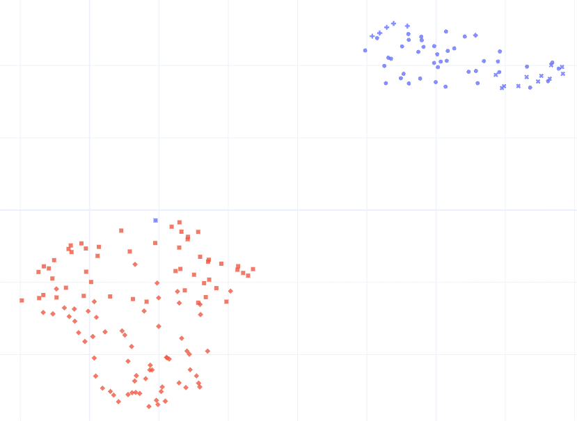
The projection layer, finding the topology: 2048 dimensions are impossible to visualize. We used UMAP to project these vectors down to just 2 dimensions. This is where the magic happens, UMAP preserves local structure, meaning if Clip A and Clip B are close to each other in the 2D plot, they're almost certainly semantically similar. When we plotted our binary classification dataset, we didn't see a random cloud of points. We saw two distinct continents, but importantly, we saw islands drifting off the coast. The blue continent, tight, dense cluster. The red continent, more spread out, representing higher variance. The outliers, a smattering of dots far away from the main clusters. When we clicked on these dots using interactive plots, they weren't our target sounds at all. They were TV static, cars driving by, or corrupted audio. We had successfully identified the garbage without listening to a single file.

For hyperparameter tuning, we found n_neighbors set to 15 helped fragment the data into many small, tight micro-clusters rather than one big continent, and min_dist set to 0.1 allowed points to pack tightly together, creating clear empty space between different types of sounds.

Interactive exploration, the tool: the final piece was interactivity. A static image of dots is interesting but not actionable, you can't debug what you can't check. We built a lightweight web-based visualisation tool where each point on the scatter plot was linked to the underlying audio file. Hover to see the filename and metadata, click to play the audio, lasso to select a group of points and export their IDs to a CSV.

# The Concept: Using geometry to clean data
svm = LinearSVC(class_weight='balanced')svm.fit(umap_2d_coords, labels)
 
# Get distance to the decision boundary
distances = svm.decision_function(umap_2d_coords)

This gave us a decision boundary, a line drawn between the two classes. More importantly, it gave us a distance metric, high positive distance means confident Class A, high negative distance means confident Class B, near zero means ambiguous or mixed. We implemented a cleaning protocol based on this geometry: remove misclassified files that fell deep into the wrong territory on the map, almost always a labeling error; and remove ambiguous files that fell within a generic threshold distance of the line, meaning the model wasn't sure. In preventive health, precision beats recall, we'd rather toss a valid file than keep a confusing one.

The results: purity by default

By applying this visual and geometric filter, we reduced our dataset size significantly, but the quality skyrocketed. When we re-ran the clustering on the cleaned dataset, the islands of noise were gone. The two continents were sharper and more distinct. We had effectively bootstrapped a high-quality dataset from scrapes without the massive overhead of manual validation. This approach fits perfectly with the clean code, clean data philosophy, instead of hoping our complex models would learn to ignore the noise, we used simpler, interpretable tools to remove the noise at the source.

Key takeaways

• Visual beats auditory.
• For large datasets, your eyes are faster than your ears, use dimensionality reduction to turn temporal data into spatial data.
• Embeddings are searchable, use pre-trained models like PANNs or CLAP as generic feature extractors, you don't need to train a model from scratch to find outliers.
• Geometry is a filter, don't be afraid to apply simple geometric rules to high-dimensional problems, sometimes a simple line in 2D space is the most robust filter you can build.
• And iterate on data, not models, improving the dataset via cleaning often yields higher accuracy gains than tweaking the hyperparameters of the final model.
• The best model architecture in the world cannot fix a dataset full of noise.
• See your data first, train second.