Introduction

Audio is one of the hardest signals to work with in real-world ML systems. Unlike images, it is continuous, noisy, and deeply tied to the environment it is captured in. At Hoomanely, we build smart pet products that live inside homes - kitchens, living rooms, and feeding areas - not controlled labs. When we started building an audio pipeline to understand dog eating behavior from our smart feeding bowl, we quickly ran into a familiar problem: not enough clean data.

We had roughly 50–60 clean, 5‑second dog eating clips. Collecting more wasn’t just slow - it was unpredictable. Classical audio augmentation helped, but often distorted the very semantics we cared about. That pushed us to explore a slightly unconventional question:

Can we safely augment audio using an autoencoder – and is that even the correct thing to do?

This post is a technical deep dive into how we trained an audio autoencoder, how augmentation actually happens, why it worked for us, and where this approach clearly fails.

The Problem: Low Data, High Variability

Dog eating audio looks simple until you listen closely. The sound changes based on:

• Bowl material and geometry (steel, ceramic, plastic)
• Microphone placement and distance
• Dog size, jaw strength, and eating speed
• Background household noise

Despite this variability, the semantic event - chewing, crunching, licking - stays consistent. Our challenge was to teach models what normal eating looks like without inventing unrealistic sounds or overfitting to a tiny dataset.

Traditional augmentations like pitch shift or time stretch often broke temporal cues. Noise mixing helped, but too much noise blurred the boundary between eating and non‑eating events.

We needed variation - but the right kind of variation.

Why We Didn’t Use Generative Audio Models

Large generative audio models are powerful, but they weren’t the right fit for our constraints:

• We didn’t need creative diversity - only robustness
• Verifying realism without labels is extremely hard
• Generative models can hallucinate events
• Edge deployment and iteration speed matter to us

Our goal wasn’t to create new dog eating sounds. It was to help downstream models tolerate real‑world variation.

This led us to a simpler idea: learn the structure of eating sounds, then perturb it carefully.

Approach: Reconstruction First, Augmentation Later

We chose a convolutional audio autoencoder trained purely for reconstruction.

Training objective:

Given a dog eating sound → reconstruct the same sound

Training setup

• Input: 5‑second clips converted to log‑Mel spectrograms
• Model: Lightweight convolutional encoder–decoder
• Loss: L1/L2 reconstruction loss (optionally spectral convergence)

The model’s job was intentionally narrow. It wasn’t asked to denoise, classify, or generate - only to compress and reconstruct eating acoustics.

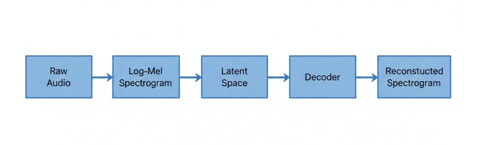
Figure 1: Training an audio autoencoder purely for reconstruction of dog eating sounds.

What the Autoencoder Learns (and Ignores)

Through reconstruction, the autoencoder consistently learned:

• Chewing rhythm and temporal envelopes
• Energy distribution across frequency bands
• Repetitive textures typical of eating

Equally important, it largely ignored:

• Exact background noise patterns
• Bowl‑specific resonances
• One‑off transient sounds

This separation is critical. It means the latent space captures what eating sounds like, not everything that happens around it.

Where Augmentation Actually Happens

A key clarification:

Augmentation does not happen during training.

Once the autoencoder converges, we generate augmented samples by slightly perturbing the latent representation during inference:

• Small Gaussian noise injection
• Partial latent dropout
• Mild decoder‑side perturbations

The output audio:

• Preserves eating semantics
• Varies surface acoustics
• Stays close to the original distribution

We refer to this as latent‑space augmentation, not audio synthesis.

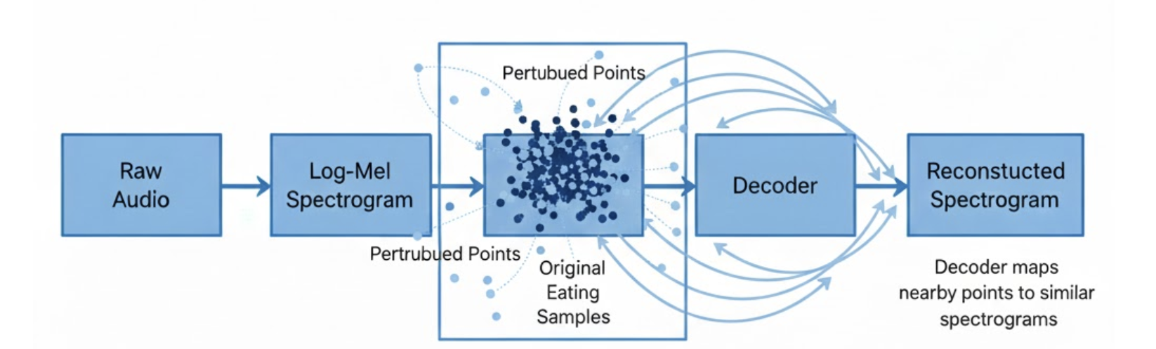
Figure 2: Latent‑space perturbations create controlled acoustic variation without changing semantics.

Why This Worked for Our Use Case

Our downstream tasks were:

• Audio embeddings
• Unsupervised anomaly detection
• Lightweight classifiers running on edge devices

For these tasks, robustness matters more than perceptual realism. The augmented samples helped models learn which variations still count as normal eating.

In embedding space, original and augmented samples clustered tightly. During real‑world testing, this translated to:

• Fewer false positives
• Better tolerance to background noise
• More stable anomaly scores

How We Validated We Didn’t Break the Signal

We didn’t judge success by listening alone. Instead, we validated downstream behavior:

• Embedding similarity between original and augmented audio
• Consistency of anomaly scores across variants
• Reduced alert noise in production‑like environments

Augmentation was only kept if it improved system‑level behavior.

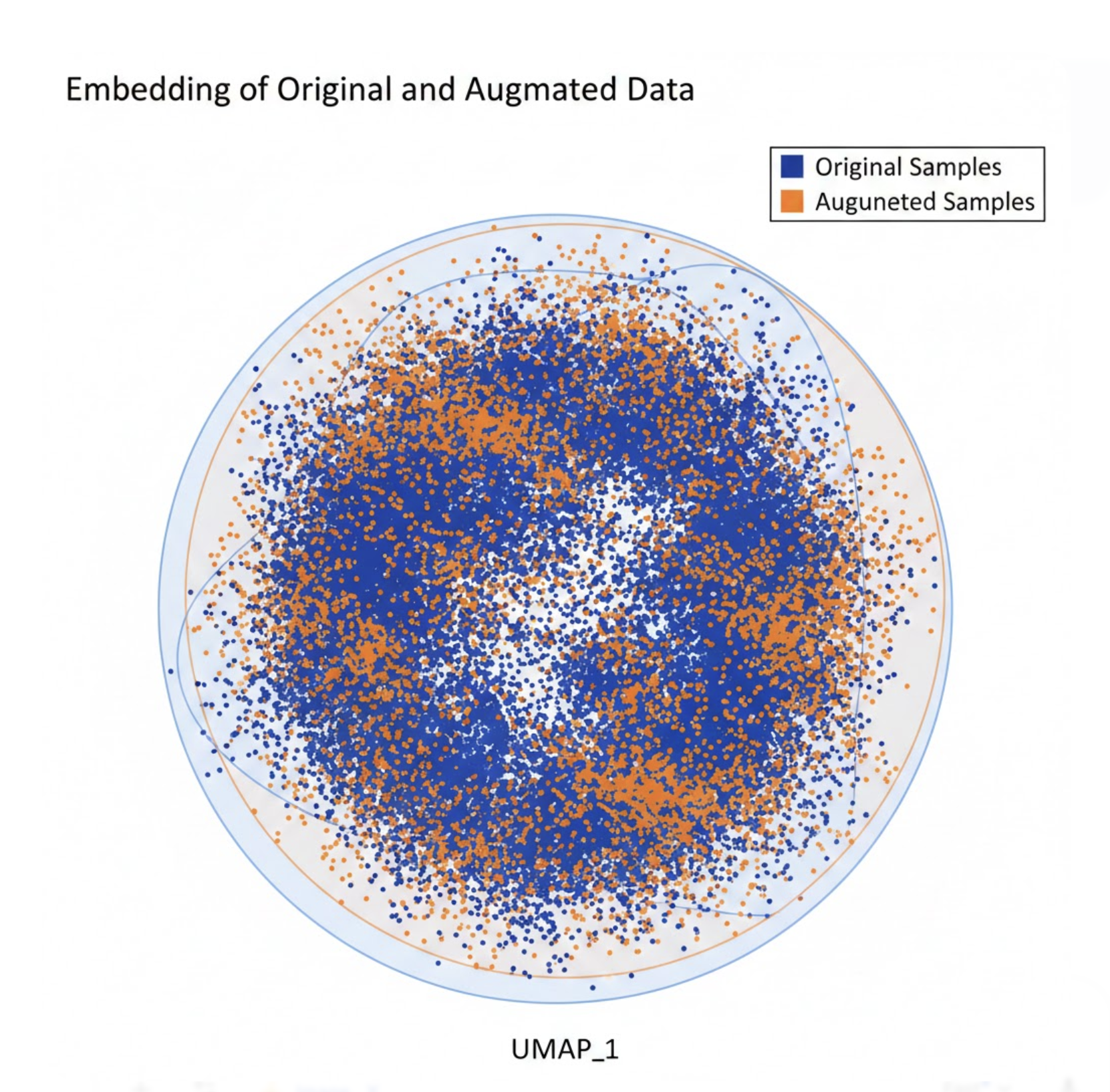
Figure 3: Augmented samples remain close to originals in embedding space.

Where This Approach Fails

Autoencoder‑based augmentation is not universally correct. It breaks down when:

• Human‑perceived realism is critical
• Precise transient timing matters
• Speech or linguistic content is involved
• Open‑ended sound generation is required

In those cases, generative or diffusion‑based models are the right tool.

Key Takeaways

• Autoencoders don’t create new sounds - they create tolerance to variation
• Latent‑space augmentation is effective in low‑data regimes
• Validation must happen at the system level, not waveform quality
• Correctness depends on alignment with the actual product goal

Autoencoders didn’t make our dataset bigger - they made our models more tolerant to reality.