Building Unsupervised Anomaly Detection for Edge Audio

When your edge device captures thousands of audio clips in real-world conditions, the question isn't just "what's happening?" — it's "what's going wrong?" At Hoomanely, our Everbowl continuously monitors a pet to provide preventive healthcare insights for pets. But audio from edge devices is messy: human voices bleed in, TV shows interfere, microphones get bumped, and background noise creates false patterns. We needed a system that could automatically surface these anomalies.

The Problem: Beyond Simple Classification

Most audio ML problems are framed as classification: "Is this a dog eating or not?" But that's not our challenge. We know most clips contain eating sounds. What we need to identify are:

Sensor failures: Clipped audio, dead channels, electrical interference
Environmental contamination: Human speech, TV audio, metallic bangs
Edge cases: Unusual eating patterns that might indicate health issues
Data quality issues: Silence-only clips, corrupted recordings

The catch? These anomalies are rare, diverse, and unlabeled. We needed unsupervised discovery, not supervised classification.

Why Traditional Approaches Fall Short

Threshold-based detection (volume, frequency bands) catches obvious failures but misses subtle anomalies like faint background speech or unusual chewing patterns.

Supervised models require extensive labeled data for every anomaly type — impractical when anomalies are long-tail and constantly evolving.

Simple clustering on raw audio features creates clusters based on loudness or duration rather than semantic content, drowning true anomalies in noise.

We needed something smarter.

The Audio Separation Challenge

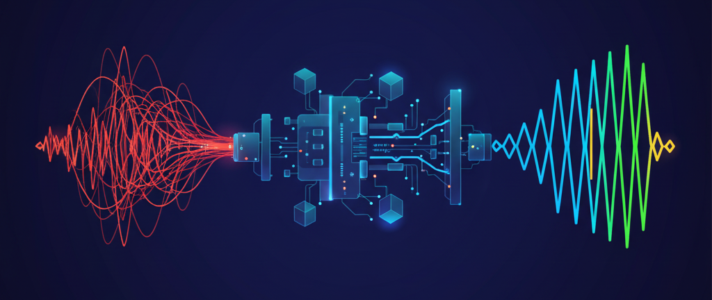
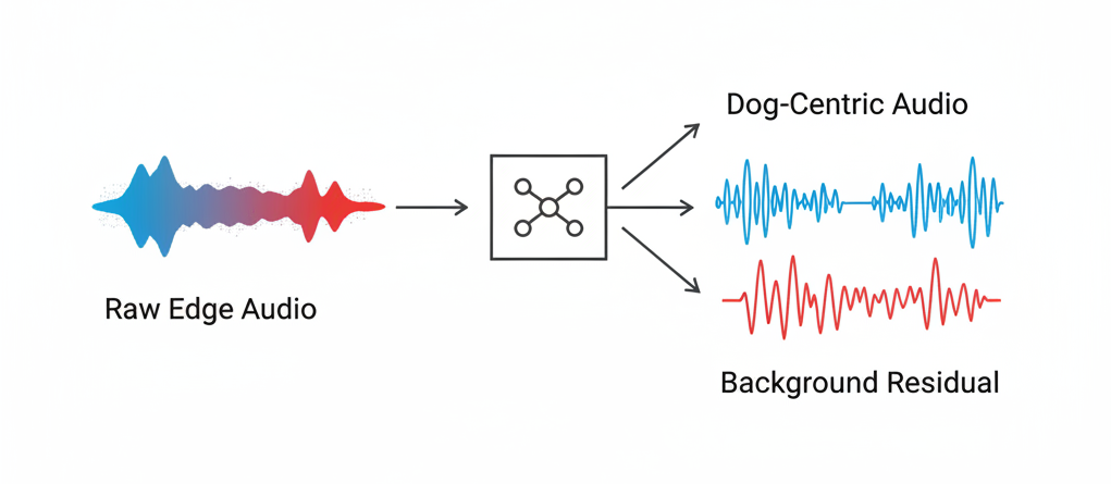
Raw edge audio is a cocktail of target sounds (dog sounds) mixed with everything else (HVAC hum, dishwasher noise, footsteps). Before detecting anomalies, we needed to separate the signal from the noise.

AudioSep: Separating Dog Sounds from Background

We integrated AudioSep, a foundation model for audio source separation, as our first processing stage. Unlike traditional signal processing approaches, AudioSep uses deep learning to isolate specific sound sources from complex mixtures.

The key insight: by producing a "dog-centric" clean track, we could make downstream anomaly detection focus on actual eating behaviors rather than background variations. We keep both the separated output and the residual (what was removed) — the residual often contains the anomalies themselves, like human speech or TV audio that AudioSep correctly identified as "not dog sounds."

This preprocessing step reduced false positives by roughly 40% in our early testing, simply by giving the anomaly detector cleaner input to work with.

Embedding Space: Choosing the Right Representation

With clean audio in hand, we needed to convert variable-length clips into fixed representations that capture acoustic similarity. This is where embedding model selection became critical.

PANNs vs. CLAP: The Trade-off Between Semantics and Acoustics

We evaluated two leading audio embedding approaches:

CLAP (Contrastive Language-Audio Pretraining): Text-aligned embeddings that excel at semantic similarity. A dog barking and a wolf howling are "close" because they share conceptual meaning.

PANNs (Pretrained Audio Neural Networks): Acoustic-texture embeddings trained on environmental sounds. A dog barking and a door slamming might be close if they share similar frequency characteristics.

For our use case, PANNs won decisively. Here's why:

CLAP's semantic alignment works against unsupervised anomaly detection. When all "dog-related" sounds cluster tightly regardless of acoustic quality, subtle anomalies (microphone rubs, distorted audio) get buried in the semantic cluster. CLAP is phenomenal for retrieval ("find all clips of dogs drinking water"), but its text-grounded geometry obscures the acoustic outliers we care about.

PANNs, on the other hand, creates embeddings based purely on acoustic texture. A clean chewing sound and a distorted chewing sound land in different regions of the embedding space — exactly what we need for anomaly detection. The 2048-dimensional embeddings from CNN14's penultimate layer gave us rich, stable representations of acoustic patterns.

Windowing: Capturing Brief Anomalies

Audio clips from our bowls range from 5 to 30 seconds, but anomalies are often brief — a 2-second burst of TV audio, a 1-second mic bump. Processing full clips would average out these signals.

We adopted 2-second windows with 1-second hop overlap. Each clip becomes a sequence of overlapping windows, and we compute embeddings per window. This granularity is critical: anomaly scores are calculated at the window level, then aggregated back to clips. It means a single 2-second anomaly in a 20-second clip doesn't get diluted — it stands out.

Dual Detection: Combining Global and Local Views

With embeddings in hand, we needed to answer: "Which windows are anomalous?" This is where the architecture gets interesting.

Why One Detector Isn't Enough

HDBSCAN (density-based clustering) excels at finding global structure. It identifies natural clusters in the data — one for chewing, one for licking, one for silence — and labels everything else as "noise." Great for catching truly weird samples that don't fit any normal pattern.

LOF (Local Outlier Factor) excels at finding local deviations. It catches samples that are odd relative to their nearest neighbors, even if they're inside a broader cluster. Perfect for subtle anomalies like a chewing sound with faint background speech.

Using both gives us coverage across anomaly types: HDBSCAN for "this doesn't fit anywhere" and LOF for "this is weird given what's nearby."

The Ensemble Strategy

For each audio window, we compute:

• HDBSCAN anomaly score: Based on whether it's labeled as noise (cluster ID = -1) and its probability of belonging to any cluster
• LOF anomaly score: Based on its local density compared to neighbors

We ensemble these with weighted combination (60% HDBSCAN, 40% LOF) and aggregate to the clip level using the maximum window score. This means if any 2-second segment in a clip is highly anomalous, the entire clip gets flagged for review.

Dimensionality Reduction with UMAP

Before feeding embeddings to HDBSCAN, we reduce from 2048 dimensions to 40 using UMAP (Uniform Manifold Approximation and Projection). This serves three purposes:

1. Speed: HDBSCAN scales poorly with dimensionality
2. Structure: UMAP preserves local and global structure better than PCA, creating cleaner density regions
3. Visualization: 2D UMAP projections let us visually inspect cluster quality and anomaly placement

Interestingly, we run LOF on the original scaled embeddings, not UMAP-reduced ones. In testing, LOF performed better with full dimensionality for local neighbor calculations, while HDBSCAN needed the structure that UMAP provides.

The Verification Loop: Measuring Success Without Full Labels

The beauty of unsupervised learning is you don't need labeled training data. The challenge? You still need to verify it's working.

Precision@K and Cluster Quality

We built a lightweight human-in-the-loop review process:

1. Sample strategically: Top 2-5% anomalies (40-100 clips), plus 20 random baseline clips and samples from each major cluster
2. Three-tier labeling: ✓ Normal dog sounds, ⚠️ Rare-but-okay , ✗ True anomaly
3. Track Precision@K: Of the top K flagged clips, what percentage are actually problematic?

Just as important: we verify cluster quality. Are normal eating patterns forming stable clusters? Are different normal behaviors (chewing vs. licking) separating naturally? This confirms the pipeline isn't just finding outliers, but understanding structure.

Tuning Based on Real Errors

The verification loop revealed specific failure modes:

Too many false positives? Increase window length to 3 seconds for more context, or reduce LOF sensitivity by increasing neighbor count.

Missing obvious glitches? Add hard filters for silence-only clips or audio clipping, which sometimes slip through embeddings-based detection.

This feedback mechanism is what transforms a research prototype into a production tool.

Key Takeaways

Audio source separation first: Cleaning the input with AudioSep reduced downstream false positives significantly. Don't skip preprocessing.

Embeddings matter deeply: Choose based on your task. Semantic embeddings (CLAP) for retrieval, acoustic embeddings (PANNs) for anomaly detection.

Dual detection covers more ground: HDBSCAN for global outliers, LOF for local deviations. One detector misses what the other catches.

Verification beats validation: You don't need thousands of labels. Strategic sampling and Precision@K gives you enough signal to tune and trust.

Window-level granularity: Brief anomalies in long clips need fine-grained analysis. Don't average them out.

Unsupervised anomaly detection isn't about eliminating human review — it's about making that review focused, efficient, and high-value. We traded blind data wrangling for targeted investigation, and that's made all the difference.