CLAP Audio Transformer as a Validator, Not a Classifier

Using large models to sanity-check edge detections

Introduction

Audio datasets are fragile. Unlike images or text, you cannot visually skim through thousands of audio samples and immediately know whether they belong to the right class. A barking dog, a metal clank, or background human speech can sound deceptively similar in short clips—especially when captured by edge devices in uncontrolled environments.

At Hoomanely, we ran into this exact problem while building audio pipelines for edge devices. Our goal was not to train a giant cloud classifier, but to build small, reliable edge models. That forced us to ask a different question:

What if large models are better used as validators rather than classifiers?

This post walks through how we scraped audio for a specific class, clustered it using embeddings from CLAP, visually inspected those clusters with UMAP, and then used CLAP again—this time with text prompts—to sanity‑check which samples were truly positive. Those validated samples became our true positives (TPs) for training lightweight edge models.

The Problem: Noisy Labels in Audio

When you scrape or aggregate audio at scale, label noise is unavoidable:

• Keyword‑based scraping pulls in unrelated sounds
• Weak labels ("dog eating", "chewing") overlap with similar classes
• Manual validation does not scale

For edge ML, label noise is especially dangerous. Small models overfit quickly, and a 10–20% contamination rate can completely collapse precision.

We needed a way to filter candidate audio—not perfectly classify it.

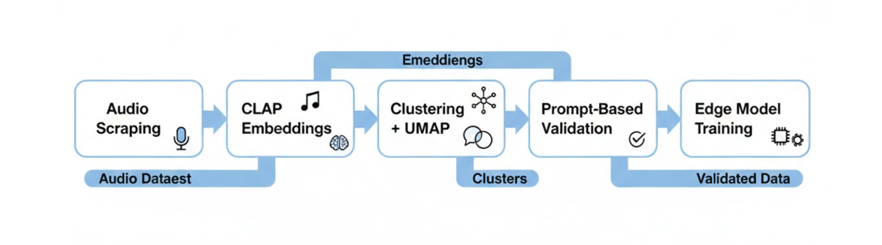
Our Approach (High Level)

We split the pipeline into four distinct stages:

1. Scrape candidate audio for a target class
2. Embed all audio using CLAP
3. Cluster and visualize embeddings with UMAP
4. Use CLAP with text prompts to validate clusters

Large models (CLAP) were only used where they are strongest: representation learning and semantic alignment.

Step 1: Scraping a Target Audio Class

We started by scraping audio for a single target class (e.g., a specific dog‑related sound). Sources included:

• Public audio datasets
• Long‑form videos split into clips
• Web‑scraped short audio segments

At this stage, we assumed the dataset was dirty by default. No attempt was made to hand‑label everything upfront.

Treat scraped audio as candidates, not ground truth.

Step 2: Creating Embeddings with CLAP

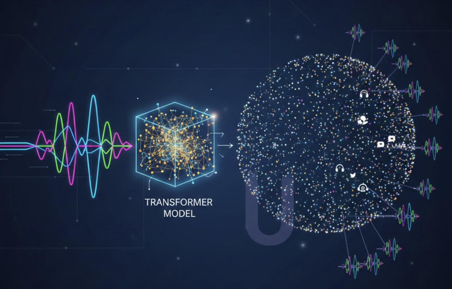
To understand the structure of the data, we embedded every audio clip using CLAP (Contrastive Language–Audio Pretraining), a transformer-based model trained jointly on audio–text pairs.

Rather than treating CLAP as a classifier, we used it purely as a representation model. Each audio clip was converted into a fixed-length embedding that captures high-level semantic information ("what the sound is about"), not low-level acoustics.

A few important implementation details worth calling out:

• Input standardization: All clips were resampled and normalized to a consistent duration and sampling rate before embedding.
• No prompt at this stage: We deliberately avoided text prompts here. The goal was to let the audio space organize itself naturally.
• Frozen model: CLAP was used fully frozen—no fine-tuning—so embeddings remained stable across experiments.

This step gave us a dense semantic space where similar sounds naturally cluster together, even when their raw waveforms differ significantly.

Why CLAP for embeddings?

• Transformer-based global context (not frame-local heuristics)
• Strong semantic separation across sound types
• Same embedding space later enables text-based validation

At this point, CLAP’s role was complete: produce embeddings we could reason about, cluster, and visualize.

Step 3: Clustering + UMAP Visualization

Once embedded, we clustered the audio embeddings using standard clustering methods (e.g., k‑means or density‑based clustering).

To see what was happening, we reduced the embeddings to 2D using UMAP.

[Image Placeholder – UMAP Cluster Plot]
Prompt: UMAP scatter plot showing multiple colored clusters of audio embeddings, some dense and compact, others sparse and isolated. Clean research-style plot, white background, minimal axis labels.

What UMAP showed us

• Dense clusters of highly similar sounds
• Isolated pockets of noise (speech, background music, artifacts)
• Mixed clusters that needed deeper inspection

This visualization step was critical. It gave us an intuition for:

• How many sub‑modes existed within a single class
• Which clusters were likely usable
• Which clusters were suspicious

Step 4: Listing and Auditing Cluster Samples

For each cluster, we randomly sampled audio clips and listened to them manually.

Instead of validating everything, we validated representatives:

• 10–20 clips per cluster
• Focus on cluster centroids

This reduced human effort by orders of magnitude while still giving confidence about cluster quality.

Clusters that were clearly off‑class were discarded early.

Step 5: CLAP as a Validator (Prompt‑Based Filtering)

Here’s the key idea: once clusters looked reasonable, we ran CLAP again, but this time in validation mode.

For each audio clip in a cluster:

• We passed a text prompt describing the target class
• Computed audio–text similarity
• Applied a conservative threshold

Only clips that strongly matched the prompt were retained.

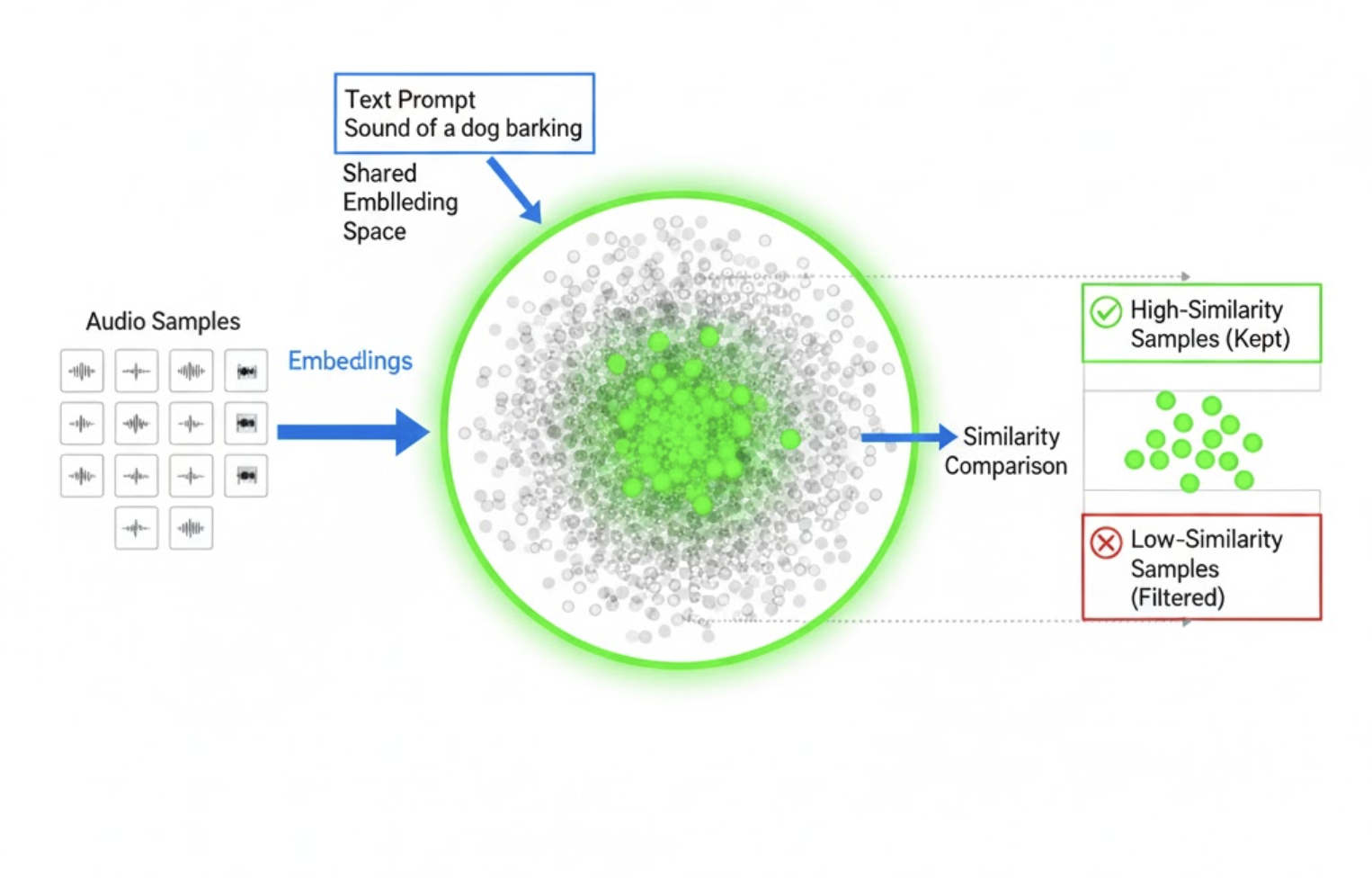
CLAP was not deciding the class—it was confirming semantic consistency.

These retained clips were treated as true positives (TPs).

Why This Works Better Than Direct Classification

Using CLAP directly as a classifier would have been simpler—but also riskier.

Classification problems:

• Thresholds are hard to calibrate
• False positives are opaque
• Errors compound silently

Validation advantages:

• Human‑interpretable prompts
• Cluster‑level sanity checks
• Conservative filtering by design

We intentionally biased toward high precision, lower recall at this stage.

Results

After validation:

• Label noise dropped significantly
• Cluster purity improved
• Edge model training stabilized

Small CNN‑based and Mel‑spectrogram models trained on this filtered data showed:

• Fewer false positives
• Faster convergence
• Better generalization on real device data

Most importantly, failures were explainable.

Key Takeaways

• Audio labels are inherently noisy—assume that upfront
• Use large models for representation and validation, not blind classification
• Clustering + visualization reveals structure humans can reason about
• Prompt‑based validation scales better than manual labeling
• High‑precision data beats large, noisy datasets for edge ML