Image Size Budgets in Embedded Systems: Pruning, Stripping & Compression for Efficient Edge Imaging

In modern imaging pipelines, especially ones running on edge devices, every byte matters. When an embedded system captures images, those images have to travel through limited memory, constrained communication buses, and strict power budgets. Large image payloads degrade system performance, slow down recovery pipelines, and create unpredictable behavior. To keep imaging fast and predictable, we define image size budgets.

Image size budgeting is the practice of controlling how large an image is allowed to be across its lifecycle, from capture through transmission to storage. At Hoomanely, while building our AI-powered smart pet bowl with a camera sensor, we learned this the hard way. Our initial implementation captured maximum-resolution images and tried to transmit them to an edge device for ML inference, and transmission took multiple seconds per frame.

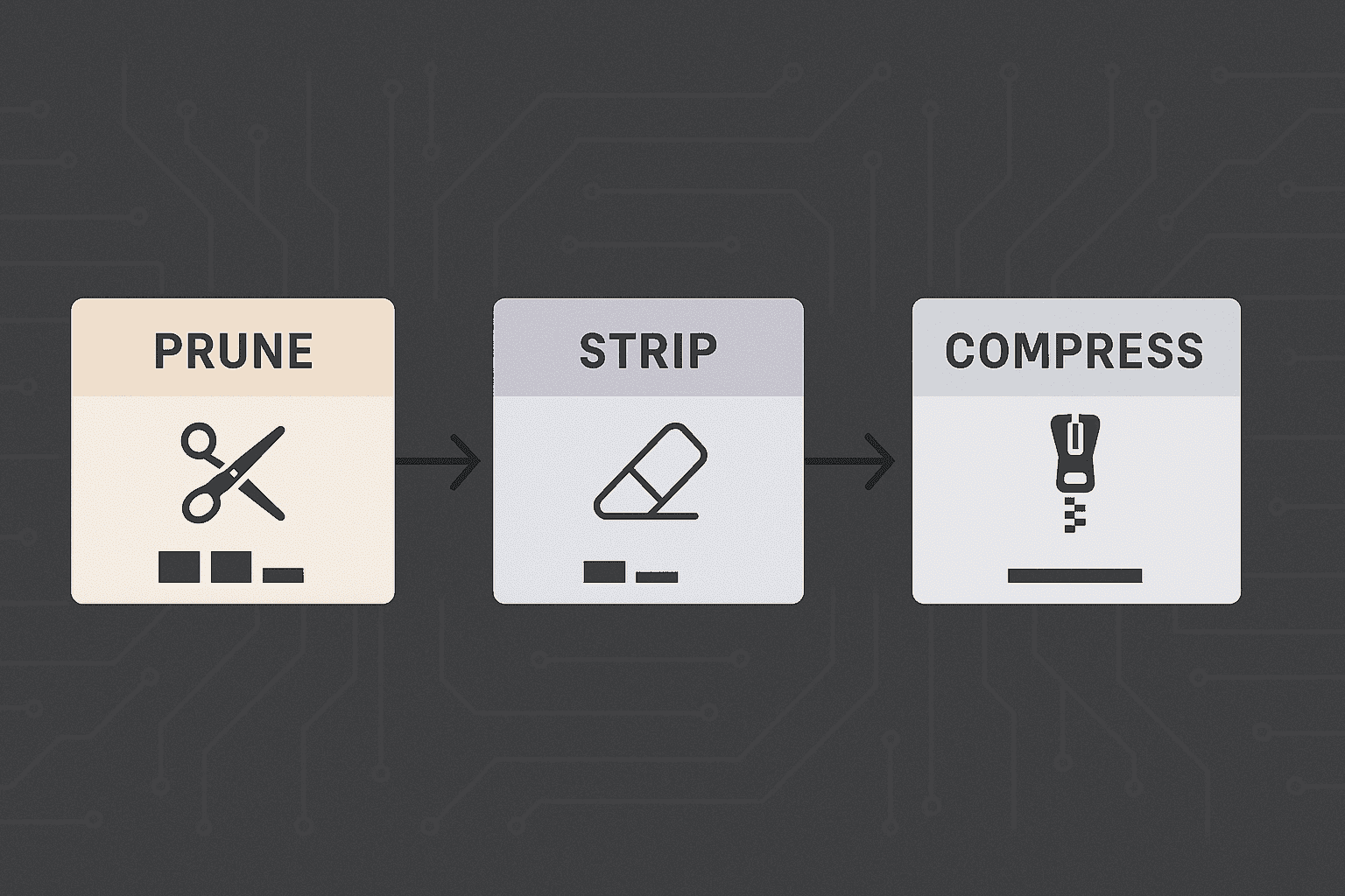
Achieving efficient imaging takes three complementary strategies applied in sequence: pruning, to minimize what you capture; stripping, to remove what you don't need; and compression, to encode what remains efficiently.

The hidden cost of uncontrolled images

In resource-constrained systems, raw, unoptimized images lead to transfer and sync times measured in minutes instead of milliseconds, unpredictable memory consumption that exhausts storage without warning, reduced throughput in recovery pipelines as bus congestion blocks critical sensor data, and increased latency on transmission paths that delays real-time inference. Each stage of the pipeline should reduce payload before the next process touches it, enabling predictable latency, controlled memory usage, and efficient recovery.

Pruning: reduce what you capture

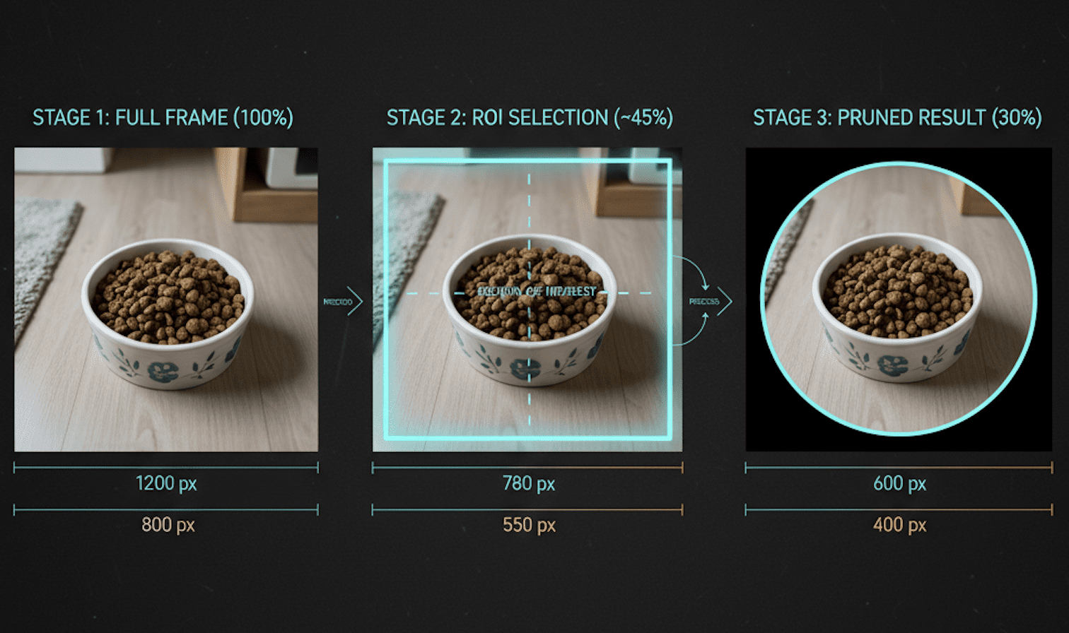
Pruning removes unnecessary image data before encoding or transmission. Instead of capturing, storing, or transmitting the entire frame, pruning forces the system to define what portion is actually useful for the task at hand. The camera sensor can capture at maximum resolution, but not every task needs that level of detail, some benefit from richer detail and color, others work fine with reduced resolution, some analyses only need grayscale, and many scenarios only need a portion of the frame.

Typical pruning operations: resolution reduction, configuring the sensor to capture only what's needed rather than maximum resolution that wastes bandwidth. Region-of-interest cropping, since our bowl occupies a fixed position in the frame, there's no reason to transmit the surrounding environment. Color-space conversion, since RGB carries full color info but water-level detection works fine in grayscale, cutting data by a third. And channel elimination, dropping alpha channels or unused color components that don't contribute to inference accuracy.

The cheapest byte is the byte never generated. Pruning happens at capture time, where the cost of moving extra pixels is highest, and every pixel that never gets captured never needs to be stored, transmitted, or processed downstream.

Stripping: remove what you don't need

After pruning cuts pixel count, the next step eliminates non-pixel overhead. Digital images carry hidden baggage that bloats file size without contributing to quality or ML accuracy: EXIF metadata (camera make and model, capture settings, timestamps, GPS coordinates, shutter speed, ISO), color profiles (ICC calibration data meant for display accuracy, irrelevant for a system that never renders images for human viewing), sensor calibration data (the AR0144 embeds color correction matrices and lens shading data that helps processing but isn't needed afterward), and debug information (thumbnails, register dumps, frame counters, useful during development, wasteful in production).

The distinction between pruning and stripping matters: pruning removes pixels and changes visual quality by design, applied at capture time; stripping removes metadata without touching a single pixel, applied after capture. Metadata overhead varies by sensor but typically adds several kilobytes per frame, and over hundreds of daily captures that compounds into megabytes of wasted storage and bandwidth. On bandwidth-constrained buses, every kilobyte saved frees capacity for other critical sensor data, weight sensors, temperature probes, proximity detectors. Stripping reduces clutter, not clarity.

Compression: make what remains efficient

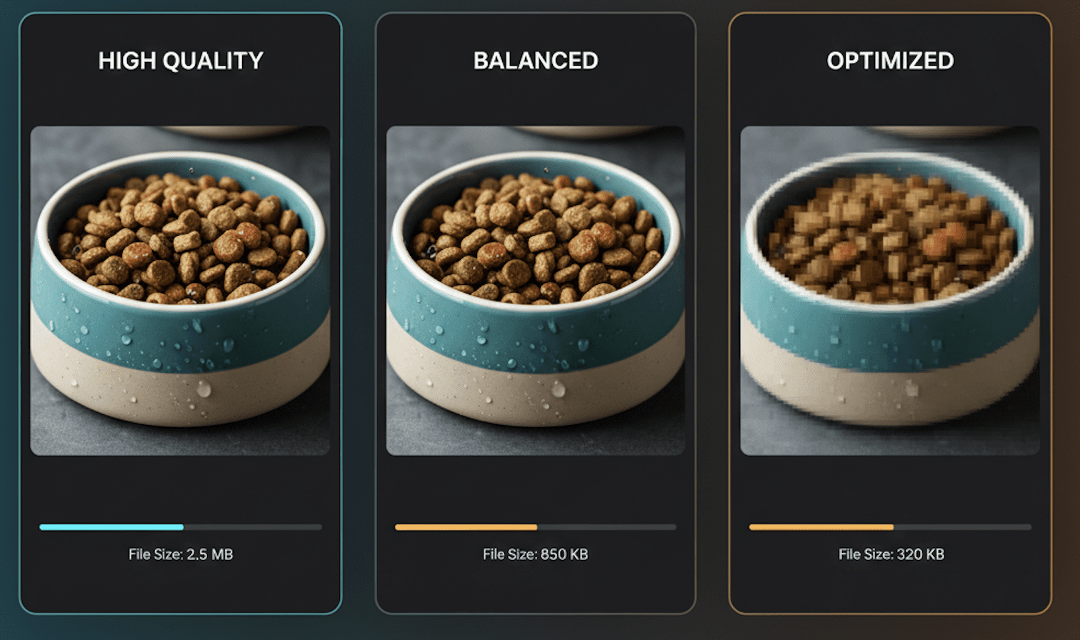
After pruning and stripping, compression reduces the size of what's left. Format selection matters here, JPEG, PNG, WebP, but the fundamental rule is that compression should only apply after pruning and stripping, compressing a full-resolution image loaded with metadata wastes effort compressing bytes you were going to throw away anyway.

Lossless compression preserves every bit, useful for debug builds, reproducibility, and exact comparisons, at the cost of larger files. Lossy compression discards perceptually insignificant information for dramatic size reduction, ideal for transmission and bandwidth-constrained channels where perfect reconstruction isn't required. Different use cases call for different compression strategies, and quality settings should adapt dynamically based on available bandwidth, urgency, and inference requirements.

The system architecture

A predictable imaging pipeline looks like this:

[ Image Capture ]
       |
[ Pruning Layer ]
   (Resolution, ROI, Color Space)
       |
[ Stripping Layer ]
   (Metadata Removal)
       |
[ Compression Layer ]
   (Format Encoding)
       |
[ Transmission ]
   (Bus, Network, Storage)

Each stage cuts payload before the next handles it, enabling predictable latency, controlled memory usage, efficient recovery pipelines, power optimization through shorter transmission windows, and more bus bandwidth for other sensors. These optimizations compound: if pruning cuts the data by one factor, stripping adds another, and compression adds yet another, the final payload can end up orders of magnitude smaller than the raw capture. This isn't clever tricks, it's intentional engineering at each pipeline stage.

When to use each technique

Use pruning when you don't need the entire scene, when smaller dimensions are acceptable for your ML model, when different contexts call for different resolutions, or when real-time performance is critical. Use stripping when pixel integrity has to stay completely untouched, when metadata offers no operational value downstream, or when storage efficiency matters over long deployments. Use compression when format compatibility is required, when network bandwidth is the primary constraint, or when transmission time directly affects user experience. The most effective pipelines combine all three, in sequence, prune first, strip second, compress last.

Results and real-world impact

After implementing this three-stage pipeline in Hoomanely's pet bowl system, transmission time dropped from several seconds to under 200 milliseconds. Bus utilization went from congested to healthy, freeing bandwidth for other sensors. Daily storage requirements dropped from hundreds of megabytes to single digits. Battery life nearly doubled thanks to shorter transmission windows. And inference latency dropped enough to enable genuinely real-time pet monitoring.

On reliability, multi-pet households no longer see collisions from simultaneous bowl transmissions, feeding notifications arrive instantly, performance stays consistent regardless of network conditions, and the system runs all day without recharging. Despite the aggressive optimization, ML model accuracy stayed high, since most computer vision models don't actually need maximum resolution to perform well, and finding the minimum acceptable quality unlocks a lot of efficiency.

Conclusion

Image size budgets turn imaging systems from unpredictable into reliable. Applying pruning, stripping, and compression in sequence builds a pipeline that respects memory constraints, transmission limitations, and power budgets while still delivering high-quality results. The lesson from building Hoomanely's pet monitoring system: constraints breed creativity. Limited bandwidth forced us to question every assumption, limited power forced us to optimize every stage, limited memory forced us to define what actually matters. If you're building embedded vision systems, IoT devices, or edge ML applications, define your image size budget early. Embrace the constraints, your users will notice the milliseconds you save.