JPEG Compression on a Microcontroller

From Raw Bayer to JPEG on STM32H5 in roughly 200ms

When a camera sensor captures an image

A camera sensor doesn't directly produce a photograph. It generates a grid of raw intensity values arranged behind a color filter mosaic. On a desktop system, converting that raw data into a JPEG is relatively straightforward.

On a microcontroller with 42KB of heap, no hardware JPEG accelerator, and a tight 200ms timing budget, the problem needs a different approach entirely. Rather than optimizing individual steps in isolation, the whole pipeline has to be designed around these constraints from the start.

Standard JPEG: a quick refresher

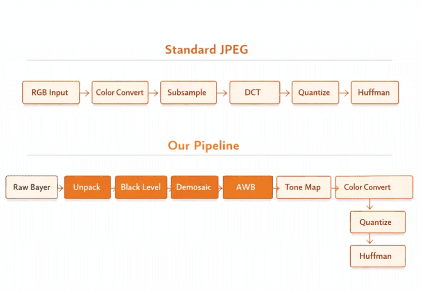
The JPEG standard assumes the input is already in RGB or YCbCr format. A typical pipeline includes RGB-to-YCbCr conversion, chroma subsampling, splitting into 8x8 blocks, the discrete cosine transform, quantization, and Huffman encoding.

Desktop implementations like libjpeg lean on floating point operations, full image buffers, and generous memory. An STM32H5 built around an ARM Cortex-M33 at 250MHz operates under significantly tighter constraints, and none of those desktop assumptions hold.

Our pipeline starts before JPEG

In this system, the input isn't a processed image, it's raw sensor data. The sensor provides 12-bit intensity values arranged in a GRGB Bayer pattern, where each pixel represents only a single color component. Getting to a JPEG means running several image signal processing steps in software before standard JPEG compression even starts.

The overall pipeline: raw Bayer, unpack, black level, demosaic, white balance, tone map, color convert, DCT, quantize, Huffman. Standard JPEG libraries aren't built to accept Bayer data, so every stage before encoding has to be implemented separately, and all of it needs to fit inside a 200ms window for a 640x400 frame.

Stage 1: unpacking 12-bit sensor data

The sensor outputs 12-bit values stored in 16-bit containers, aligned to the most significant bits. That format lets unpacking happen with a direct memory copy. Alternative packed formats, like tightly packed 10-bit or 12-bit layouts, require bit-level extraction and add overhead. Choosing the right sensor output format up front avoids that cost entirely.

Stage 2: black level subtraction

Image sensors typically report a non-zero value even with no light hitting them. That offset, the optical black level, has to come out before anything else happens. On the Cortex-M33, the USUB16 DSP instruction processes two 16-bit pixels at once. Packing pixel values into a 32-bit register lets subtraction run in parallel, cutting the instruction count per row.

Stage 3: demosaicing

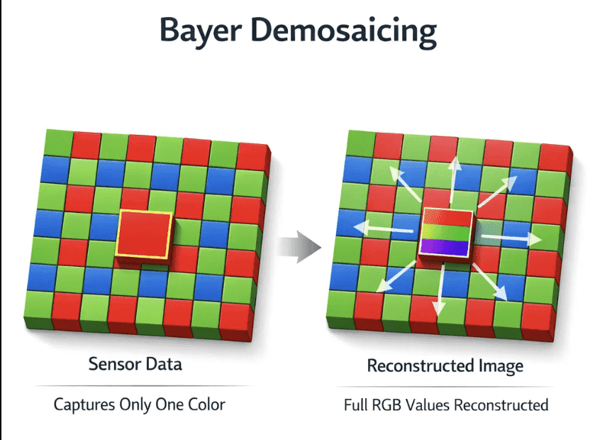
Since each Bayer pixel carries only one color component, demosaicing reconstructs full RGB values. A naive implementation would allocate a full RGB buffer, 640 x 400 x 3 bytes, roughly 768KB. That's not practical on this platform.

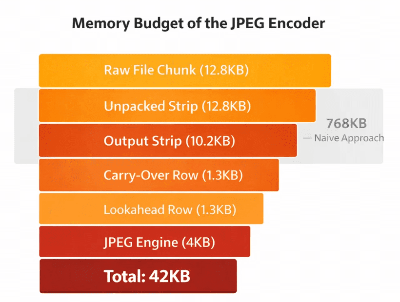
Instead, the image processes in strips of 8 to 16 rows. Each strip gets demosaiced and passed directly to the JPEG encoder. To stay correct at strip boundaries, a small number of carry-over and lookahead rows get retained. This drops memory usage from hundreds of kilobytes to roughly 13KB.

For most pixels, interpolation runs on shift-based averaging. Edge pixels take a more general path, though they're a small fraction of the image. The Bayer pattern lookup is precomputed to avoid branching in the inner loop.

Stage 4: fixed-point white balance

White balance is often implemented with floating point multiplications. Here we use Q8 fixed-point arithmetic instead. A gain of 1.375 becomes 352; 1.200 becomes 307. Each operation reduces to an integer multiplication followed by a right shift, avoiding floating point overhead while keeping enough precision for 8-bit output.

Stage 5: tone mapping

Tone mapping, gamma correction plus contrast adjustment, runs through a precomputed lookup table with 256 entries encoding the target tone curve: a gamma of 0.92 and contrast adjustment around a midpoint of 128. At runtime, tone mapping reduces to a single lookup per pixel.

Stage 6: color conversion with DSP

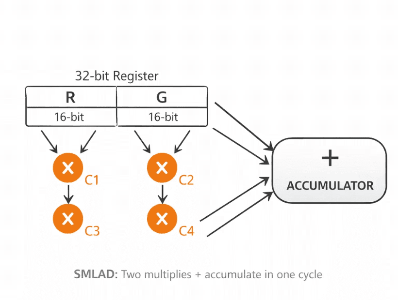
Converting RGB to YCbCr involves several multiply-accumulate operations. The Cortex-M33 provides DSP instructions like SMLAD, which perform two 16-bit multiplications and an accumulation in a single cycle. Packing color components into registers lets parts of the conversion run more efficiently, cutting the overall instruction count.

JPEG core: division-free quantization

Standard JPEG quantization relies on division, which is relatively expensive on embedded processors. Here, division gets replaced with reciprocal multiplication. Each quantization entry includes a precomputed reciprocal, letting division get approximated with a multiply and a shift. Blocks with minimal high-frequency content can also be detected and partially skipped during encoding, cutting work for smoother regions of the image.

DCT: integer implementation

The discrete cosine transform runs on integer arithmetic with Q8 scaling. Example constants: 181 for 1/sqrt(2), 98 for cos(3*pi/8), 334 for cos(pi/8). All intermediate values fit inside 32-bit integers, avoiding the overhead of mixed-width operations.

Huffman encoding optimization

A 2048-entry lookup table resolves both magnitude and sign for coefficients in one step. That avoids conditional branching for negative values and keeps the pipeline running smoothly. In practice, this cuts encoding time noticeably.

Memory budget

The full pipeline runs inside roughly 42KB: a 12.8KB raw input strip, a 12.8KB unpacked strip, a 10.2KB output YCbCr strip, a 1.3KB carry-over row, a 1.3KB lookahead row, and 4KB of JPEG engine state. A naive full-frame RGB buffer would have needed about 768KB.

Timing breakdown

Demosaic, white balance, and tone mapping together take about 45 percent of the budget. DCT and quantization take about 25 percent. Color conversion takes about 12 percent. Huffman encoding takes about 10 percent. Unpacking and black level take the remaining 8 percent. Total processing time lands around 200ms for a 640x400 image.

Key takeaways

This implementation combines a software ISP with a JPEG encoder in a single pipeline. Floating point operations stay out of performance-critical paths. Full-frame buffers aren't required anywhere. Division disappears from quantization. Branching stays minimal in the encoding stages. DSP instructions get used wherever they help. Processing happens in a streaming manner throughout.

The result is a complete raw-to-JPEG pipeline running inside tight memory and timing constraints.

Closing

Getting JPEG compression working on a microcontroller has less to do with optimizing individual stages and more to do with structuring the entire pipeline carefully from the start. A streaming approach, where data flows continuously through each stage, is what makes both memory efficiency and predictable performance possible at the same time.