Neural Network on the Camera Module
For a camera that watches a pet, the hard question is not "can it take a picture" but "can it understand one before the picture leaves the device." Our new camera module carries a dedicated neural accelerator next to its image pipeline, and on the day described here it ran its first real network: a pretrained image classifier, compiled for the accelerator, executed on a live 224×224 tile straight out of the hardware pipeline.
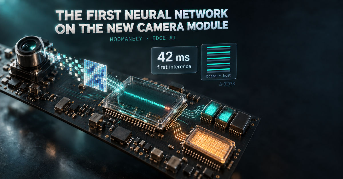
The first inference took 42 milliseconds. Its five highest-scoring classes matched a desktop reference run on the same tile, in the same order, with a worst-case difference of 0.078 in the output. Thirty of the model's thirty-two stages ran on the accelerator; the other two ran on the CPU. This post covers how the model was compiled, where it lives in memory, how it was verified, and how we are choosing the model that comes next.
The Problem: A Camera That Has to Think Locally
A pet-monitoring camera cannot stream video to a server and wait for an answer. Bandwidth, privacy, and latency all argue for the opposite: decide on the device, and send only what the decision justifies. That means a neural network has to run on a microcontroller-class part, inside a power and memory budget that a laptop would find comical.
The new camera module was chosen precisely because it includes a neural accelerator alongside the hardware image pipeline described in an earlier post. The pipeline already produces a 224×224 RGB tile with no CPU involvement. The missing piece was everything after that: a model, compiled for the accelerator, placed in memory the accelerator can reach, invoked from firmware, and proven to produce the same numbers a trusted desktop runtime produces.
"Proven" is the operative word. An accelerator that runs fast and answers wrong is worse than no accelerator at all, because it is convincing. The bring-up plan therefore treated the first inference as a measurement, not a demo.
The Approach: Compile for the Accelerator, Not the CPU
The vendor's edge-AI toolchain takes a quantized TensorFlow Lite model and emits C code plus a weight blob targeted at the accelerator. What it emits depends on two inputs we control: a compile profile and a memory-pool description. The profile selects the optimizer flags; the memory pool tells the compiler which physical memories exist, how fast they are, and what each one is allowed to hold.
The profile we settled on is the toolchain's advised minimum plus size and scheduling optimizations:
12			"default" : {
14	            "options": "--native-float --cache-maintenance --Ocache-opt --enable-virtual-mem-pools --Os --Oauto-sched"
15			},
(Line 13, which names the memory-pool file path, is omitted.)
Two of those flags matter more than they look. Cache maintenance makes the generated code clean and invalidate the CPU caches around every accelerator transfer, which is what keeps the two sides seeing the same bytes. Virtual memory pools let the compiler spill activations across several physical SRAM banks as if they were one.
The firmware side builds the accelerator runtime in polling mode with the toolchain's software fallback enabled, so any operator the hardware cannot execute still runs, on the CPU, inside the same inference call. That decision shows up directly in the epoch table later.
The Process
Carving the memory map
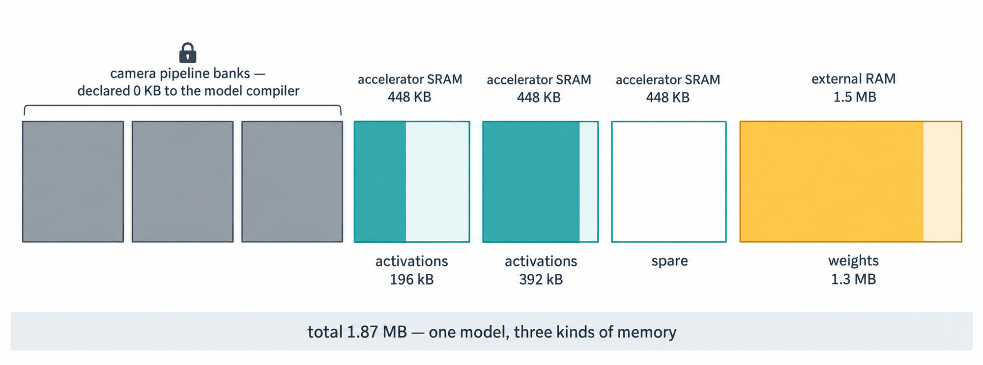
The memory-pool file is where the camera pipeline and the accelerator negotiate. The pipeline already owns several SRAM banks for its frame buffers, so those are declared to the model compiler with a size of zero: present, but off limits. Three accelerator banks are offered in full:
51				{
52					"fname": "AXISRAM4",
53					"name":  "npuRAM4",
54					"fformat": "FORMAT_RAW",
55					"prop":	  { "rights": "ACC_WRITE", "throughput": "HIGH", "latency": "LOW", "byteWidth": 8, "freqRatio": 1.25, "read_power": 18.531, "write_power": 16.201 },
56					"offset": { "value": "0x34270000", "magnitude":  "BYTES" },
57					"size":   { "value": "448",        "magnitude": "KBYTES" }
58				},
Weights are a different matter. At 1.3 MB they will not fit in on-chip SRAM beside the activations, so the external RAM is declared with a hint that constants belong there:
75				{
76					"fname": "PSRAM",
77					"name":  "psram",
78					"fformat": "FORMAT_RAW",
79					"prop":	  { "rights": "ACC_WRITE", "throughput": "MID", "latency": "HIGH", "byteWidth": 2, "freqRatio": 5.00, "cacheable": "CACHEABLE_ON","read_power": 380, "write_power": 340.0, "constants_preferred": "true" },
80					"offset": { "value": "0x70E00000", "magnitude":  "BYTES" },
81					"size":   { "value": "1536",         "magnitude": "KBYTES" }
82				},
The compiler's own report confirms the split landed exactly as intended. Activations occupy two of the three accelerator banks, weights occupy the external RAM, and nothing touched the banks the camera pipeline reserved:
129		npuRAM4    [0x34270000 - 0x342E0000]:    196.000 kB /    448.000 kB  ( 43.75 % used) -- weights:          0  B (  0.00 % used)  activations:    196.000 kB ( 43.75 % used)
130		npuRAM5    [0x342E0000 - 0x34350000]:    392.000 kB /    448.000 kB  ( 87.50 % used) -- weights:          0  B (  0.00 % used)  activations:    392.000 kB ( 87.50 % used)
131		npuRAM6    [0x34350000 - 0x343C0000]:          0  B /    448.000 kB  (  0.00 % used) -- weights:          0  B (  0.00 % used)  activations:          0  B (  0.00 % used)
132		psram      [0x70E00000 - 0x70F80000]:      1.299 MB /      1.500 MB  ( 86.60 % used) -- weights:      1.299 MB ( 86.60 % used)  activations:          0  B (  0.00 % used)
...
135	Total:                                             1.873 MB                                  -- weights:      1.299 MB                  activations:    588.000 kB
Thirty of thirty-two stages on silicon
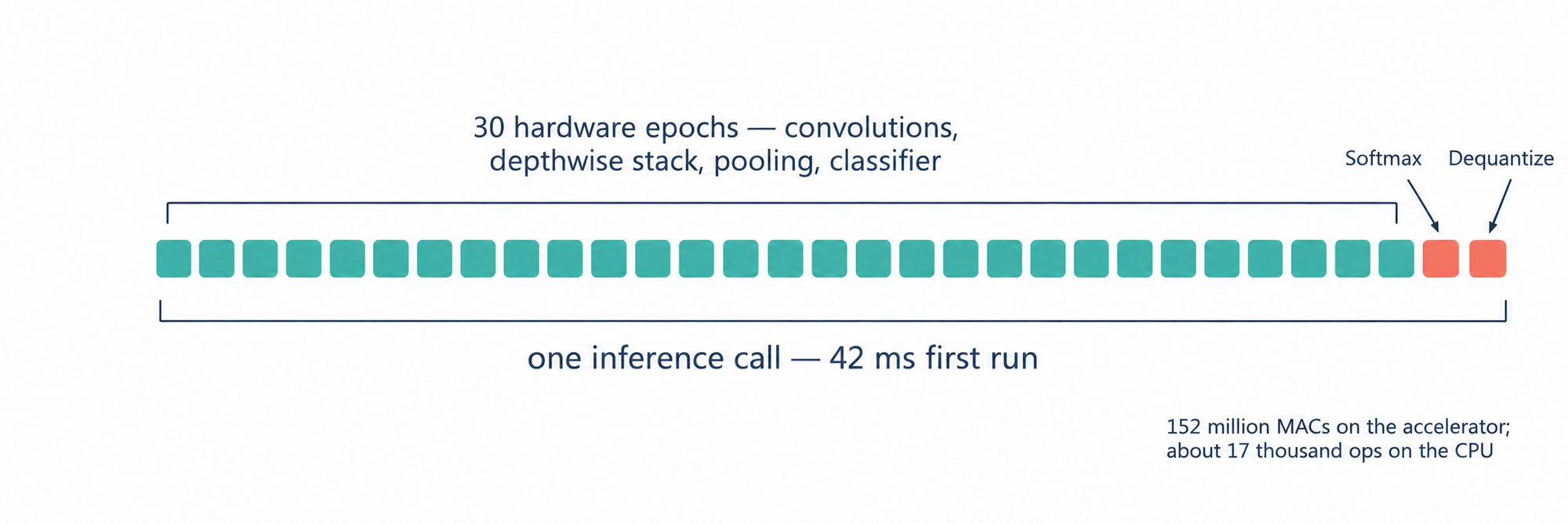
The compiler breaks the network into epochs, each a chunk of work handed to the accelerator or, when no hardware operator exists, to the CPU. The report for this model is unambiguous:
148	Total number of epochs                               32
149	>> pure software (SW) epochs                          2
150	>> hybrid epochs (using both software and hardware)   0
151	>> pure hardware (HW or EC) epochs                   30  (implemented in 0 epoch controller blobs/meta epochs)
The two software epochs are the last two in the graph:
186	| epoch_32 |  SW  |     Softmax      |
187	| epoch_33 |  SW  | DequantizeLinear |
That is exactly the right place for software. Every convolution, the depthwise stack, the pooling and the final classifier all run on the accelerator. What falls back to the CPU is a thousand-element softmax and a conversion of a thousand integers to floats: about seventeen thousand operations against the 152 million multiply-accumulates in the convolutions. The generated header fixes the interface the firmware programs against, one 150,528-byte input tile and one 4,000-byte float output:
30	#define LL_ATON_DOGNET_IN_NUM        (1)    // Total number of input buffers
31	// Input buffer 1 -- Input_0_out_0
32	#define LL_ATON_DOGNET_IN_1_ALIGNMENT   (32)
33	#define LL_ATON_DOGNET_IN_1_SIZE_BYTES  (150528)
34
35	/************************** OUTPUTS *******************************************/
36	#define LL_ATON_DOGNET_OUT_NUM        (1)    // Total number of output buffers
37	// Output buffer 1 -- Dequantize_135_out_0
38	#define LL_ATON_DOGNET_OUT_1_ALIGNMENT   (32)
39	#define LL_ATON_DOGNET_OUT_1_SIZE_BYTES  (4000)
The input size is 224 × 224 × 3 bytes, which is precisely what the hardware image pipeline already writes. No resize, no format conversion, no CPU copy sits between the sensor and the network.
Checking the board against the host
Speed means nothing without agreement, so the bench has a desktop reference. A small script runs the identical quantized model, in the standard interpreter, on the identical raw tile that the board fed its accelerator, and prints the same numbers the board prints:
14	x=raw if i['dtype']==np.uint8 else (raw.astype(np.int16)-128).astype(np.int8)
15	it.set_tensor(i['index'],x); it.invoke()
16	y=it.get_tensor(o['index']).astype(np.float32).reshape(-1)
17	sc,zp=o['quantization']
18	yf=(y-zp)*sc if sc else y
19	top=np.argsort(-yf)[:5]
20	print('host top-5 (class:value*1000):',' '.join(f'{c}:{int(round(yf[c]*1000))}' for c in top))
When the board's float output is saved and passed in, the script also prints the largest element-wise difference between the two:
23	if len(sys.argv)>2:
24	    b=np.fromfile(sys.argv[2],dtype=np.float32)
25	    print('board top-5:',' '.join(f'{c}:{int(round(b[c]*1000))}' for c in np.argsort(-b)[:5]),'| max |board-host| =',float(np.abs(b-yf).max()))
The bench log from the first successful run records both sides:
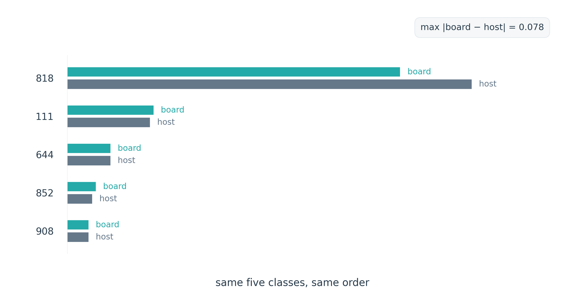
2	board: 42 ms, top-5 818:363 111:94 644:47 852:31 908:23
3	host TFLite same tile: 818:441 111:90 644:47 852:27 908:23, max |delta| 0.078
Same five classes, same order, and a worst-case difference under eight hundredths on a softmax-scale output. The residual is what you expect when the accelerator's integer arithmetic and a desktop interpreter round differently through thirty layers. More importantly, it is a number we can watch: if a future build changes the cache handling or the memory layout and that delta jumps, the bench will say so before anyone trusts a result.
Choosing the model on our own scenes
The classifier used for bring-up is a public, half-width MobileNet trained on a general image dataset. It proves the path works, but it was never going to be the production model. Rather than guess at a replacement, the bench sweeps every pretrained classifier in the local model zoo against tiles captured by our own camera, in our own lighting, and reports a single "dog" score alongside the model's size:
13	    row=f'{os.path.basename(m)[:-7]:34s} {os.path.getsize(m)/1e6:4.1f} MB'
14	    for tn,t in tiles:
15	        x=t if (h,w)==(224,224) else np.array(tf.image.resize(t,(h,w))).astype(np.uint8)
16	        if i['dtype']==np.int8: x=(x.astype(np.int16)-128).astype(np.int8)
17	        it.set_tensor(i['index'],x[None]); it.invoke()
18	        y=it.get_tensor(o['index']).astype(np.float32).reshape(-1); sc,zp=o['quantization']
19	        p=(y-zp)*sc if sc else y
20	        n=p.size; off=1 if n==1001 else 0
21	        dog=p[151+off:269+off].sum(); c=int(np.argmax(p))-off
Line 21 is the heart of it: the dataset's roughly 120 dog breeds occupy a contiguous block of class indices, so summing that block gives a breed-independent "is this a dog" probability. The sweep on a captured tile of a toy beagle, before and after colour correction, is blunt and useful:
2	mobilenetv1_a050_224_int8           1.5 MB | tile_BA.rgb    dog 0.02 top jack-o'-lantern    0.25 | tile_BA_fixed. dog 0.01 top bathing_cap        0.10
7	mobilenetv2_a140_224_int8           6.8 MB | tile_BA.rgb    dog 0.03 top bath_towel         0.10 | tile_BA_fixed. dog 0.58 top pug                0.32
The bring-up model does not see a dog in that tile. A larger model does, but only once the tile has been white-balanced and gamma-corrected. A second script then rotates a captured tile through the four right angles, with and without colour correction, to separate what the model can do from what the camera is handing it:
9	raw=np.fromfile(sys.argv[1],dtype=np.uint8).reshape(224,224,3).astype(np.float32)
10	wb=raw*(raw.mean()/raw.reshape(-1,3).mean(0)); fixed=255*(wb/max(wb.max(),1))**(1/2.2)
1	ours mnv1-0.5  captured  | rot  0: dog 0.13 wing             | rot 90: dog 0.57 golden_retriever | rot180: dog 0.10 tiger_shark      | rot270: dog 0.02 great_white_shar
4	mnv2-1.4       corrected | rot  0: dog 0.52 chow             | rot 90: dog 0.74 golden_retriever | rot180: dog 0.70 golden_retriever | rot270: dog 0.64 golden_retriever
Two things fall out of those four rows. The sensor is mounted sideways relative to how the training images were taken, and a quarter turn moves the bring-up model's dog score from 0.13 to 0.57 on the same pixels. And a model with enough capacity, fed a corrected tile, is rotation-tolerant where the small one is not. Both findings are now requirements on the next iteration, for the pipeline's orientation and colour stages as much as for the model choice.
The Results
The camera module now runs a neural network end to end on silicon: a hardware image pipeline produces the tile, a compiled model consumes it on the accelerator, and the firmware receives a thousand floats it can act on. The first inference completed in 42 milliseconds and agreed with a desktop reference to within 0.078 across every output. Thirty of thirty-two epochs execute in hardware, and the memory split keeps the camera's own buffers untouched.
Just as important is the apparatus around that number. A host-reference script that reproduces the board's computation on a desktop, a model sweep that scores candidates on our own scenes, and a rotation test that isolates mounting and colour from model capacity together turn "it works" into a repeatable measurement. The production model will be pet-specific and smaller than the general classifiers in the sweep; when it arrives, the same three tools will judge it.
Why It Matters at Hoomanely
Hoomanely is reinventing healthcare for pets — replacing reactive, imprecise care with continuous, clinical-grade monitoring that catches problems early. Our devices form a Physical Intelligence ecosystem: sensors fused at the edge, feeding the Biosense AI Engine that turns raw signals into personalized, preventive insights.
A camera that understands a frame before it leaves the device changes what the product can promise. It can decide locally whether a pet is present, which pet it is, and whether the moment is worth recording, without streaming a home to the cloud. That is better for privacy, better for bandwidth, and fast enough to react while the moment is still happening.
The engineering value is in the discipline, not just the milestone. Compiling for an accelerator, carving a memory map so two hardware blocks coexist, and refusing to trust a result until a reference agrees with it are the habits that let a small team put real intelligence into a device that lives in someone's kitchen for years.
Key Takeaways
- Treat the first inference as a measurement. Speed is easy to show; agreement with a trusted reference on the same input is what makes a result usable.
- The memory-pool file is a contract. Declaring the camera's banks as zero-size and marking external RAM as constants-preferred let the compiler place 1.3 MB of weights and 588 kB of activations without touching the pipeline.
- Read the epoch table. Thirty hardware epochs and two software ones tell you exactly what the accelerator does and what the CPU will be asked to finish.
- Sweep models on your own scenes. A breed-block dog score across the whole model zoo, on tiles from our own sensor, beats any benchmark table.
- Separate the camera from the model. A rotation-and-colour test revealed a sideways mount and a lighting correction that no amount of model shopping would have fixed.
Author's Note
This is the first network the new camera module has ever run, and it is a public classifier chosen to prove the path rather than to ship. The pet-specific model comes next, and it will be judged by the same bench: the same reference script, the same sweep, the same rotation grid. The 42 milliseconds are satisfying; the 0.078 is the number I actually care about.