Software

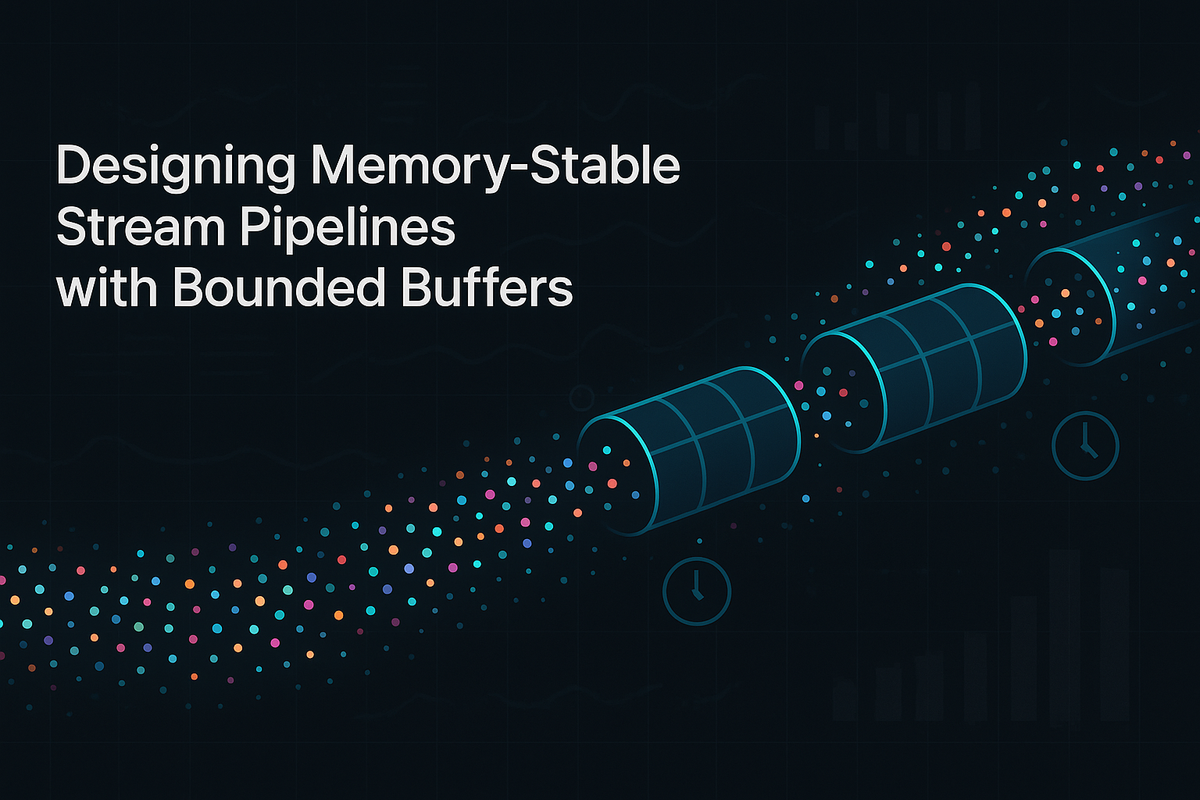
Designing Memory-Stable Stream Pipelines with Bounded Buffers

Pravin Kumar

14 Nov 2025 — 9 min read

When a streaming backend is designed well, it feels effortless: memory stays flat, latency is predictable, and reconnect storms are just another Tuesday. Even as traffic grows and features pile up, the pipeline keeps behaving like a well-tuned instrument instead of a fragile chain of patches.

A pattern that consistently delivers that kind of stability in real-time, event-driven Python systems combines bounded ring buffers, interval-driven coalescing, and timestamp-aligned batching. Together, they provide explicit memory limits, stable and predictable latency, and graceful handling of reconnects and bursts—whether the events are IMU samples from a wearable, weight readings from a smart bowl, or telemetry from long-lived app sessions.

Why Stream Backends Drift into Trouble

The healthiest stream backends aren’t defined by how they handle explosions—they’re defined by how they handle the subtle stuff.

Unbounded queues and invisible memory creep

Ingestion layer receives events (HTTP POST, WebSocket, MQTT, etc.).
Each event is appended into an in-memory list or queue.
A background worker periodically drains that structure and writes to storage.

This feels fine in development. Then production happens:

A few devices reconnect and replay buffered data.
Network hiccups cause short, high-intensity bursts of traffic.
Product features gradually increase the event rate per device.

If that buffer is unbounded, your memory usage is now a function of:

Burst size
Worker throughput
How long issues go unnoticed

By the time you see “RSS steadily climbing” in your graphs, the process is often one reconnect storm away from getting killed.

Timing drift and fuzzy batching

Another subtle failure: time drift between how you think batching works and how it actually behaves.

In production:

The worker sometimes starts late.
Processing time varies with payload size.
Load patterns change across the day.

Your “5 second” cadence turns into “somewhere between 3 and 15 seconds”, which breaks assumptions for:

User-facing freshness (dashboards, health tiles, “last updated” indicators).
Downstream analytics that expect stable windows.
Alert logic that assumes consistent latency bounds.

Reconnect storms and replays

With mobile clients, wearables, or smart devices, reconnect storms are normal:

Devices move through patchy coverage.
Apps are killed and relaunched by the OS.
Firmware buffers and replays events after outages.

If your pipeline isn’t explicit about per-device limits and what to do with replays, a reconnect storm can:

Inject a large backlog of “old” events into your hot path.
Starve fresher, more relevant data.
Inflate the memory footprint and processing time for every tick.

The smell in observability

Memory graphs that never fully flatten after load spikes.
Latency spikes that align with “a spike in active sessions”.
Coalescing or flush jobs whose run duration varies wildly.

The Pattern: Bounded, Time-Aware Stream Processing

The architecture we want can be summarized in three ideas:

Bounded per-stream ring buffers
Interval-driven coalescing (a metronome)
Timestamp-aligned batching (stable windows)

This gives you explicit control over:

How much history you keep in memory.
When work happens.
How events map into logical time windows.

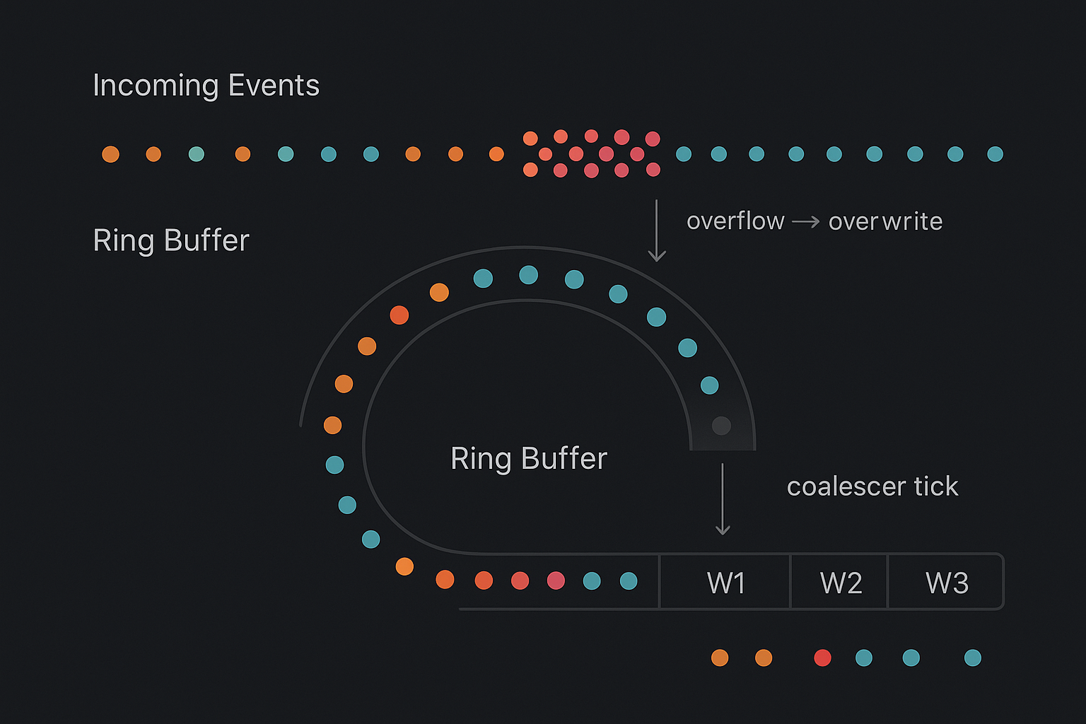
Bounded ring buffers: explicit memory budgets

For each logical stream (e.g., device_id, user_id, bowl_id), maintain a fixed-capacity ring buffer:

Capacity is expressed as “N most recent events”.
When full, new events replace or evict older ones according to a policy.

from collections import deque
from dataclasses import dataclass
from typing import Any

@dataclass
class Event:
    ts: float       # event timestamp in seconds (device or server time)
    payload: Any

class RingBuffer:
    def __init__(self, capacity: int):
        self.capacity = capacity
        self._data = deque(maxlen=capacity)

    def append(self, event: Event):
        self._data.append(event)  # oldest entries overwritten automatically

    def snapshot(self) -> list[Event]:
        return list(self._data)   # shallow copy for safe iteration

Per-stream memory usage becomes:

max_events_per_stream = capacity
max_events_overall = capacity * active_streams

Now you can reason about RAM in advance, instead of discovering it in your alerts.

Interval-driven coalescer: the metronome

Instead of “flush whenever enough events accumulate”, you introduce a coalescer loop that fires at a fixed interval (e.g., every 2–5 seconds):

At each tick:
- Snapshot the buffers.
- Partition events into windows.
- Build batches.
- Emit them to storage or downstream services.

This gives you:

Predictable CPU utilization and I/O patterns.
A natural place to enforce cluster-wide constraints.
A clean mental model: “every interval_s, each active stream gets processed”.

async def coalescer_loop(buffers, window_s: int, interval_s: float):
    while True:
        now_ts = time()
        batches = build_batches(buffers, window_s, now_ts)
        for batch in batches:
            await emit_batch(batch)  # write to DB, queue, or cache
        await asyncio.sleep(interval_s)

Timestamp-aligned batching: windows you can reason about

Instead of “whatever arrived between ticks”, we align events to explicit time windows:

Fixed size: e.g. 5 seconds, 30 seconds, or 1 minute.
Derived from event timestamps (event time) or arrival time.

Windows then become first-class:

window_id → [t_start, t_end)
Stored alongside aggregates.
Used as keys in databases or downstream queries.

This is essential for:

Time-series analytics.
ML feature engineering (e.g. “features per 5-second window”).
Consistent user-facing updates (“this card refreshes every 10s window”).

Implementation Process in Python

Let’s turn the pattern into a concrete pipeline you can integrate into a real backend, Assumptions:

A Python service receives events via HTTP or WebSockets.
Events are tagged with a stream identifier (stream_id) and timestamp.
We maintain in-memory bounded buffers and periodically persist windowed batches to storage (e.g., DynamoDB, Postgres, or a time-series DB).

Step 1 — Define your time semantics

Two key decisions:

Window size
- Short windows (e.g. 5s) → fresher UI updates, more batches.
- Longer windows (e.g. 30–60s) → fewer writes, coarser granularity.
Time source
- Event time (device timestamp) for analytics and ML.
- Arrival time (server timestamp) for freshness and alerting guarantees.

You can store both, but pick one as the canonical dimension for batching. For many health or telemetry systems, event time windows with arrival time SLAs is a good compromise.

Step 2 — Size ring buffers from traffic and SLAs

Estimate per-stream peak:

r = maximum events/second/device you’re willing to support.
H = horizon (seconds of history) you want to keep in memory.

Approximate capacity: capacity_per_stream ≈ r * H

Up to 40 events/s from a device (e.g., IMU samples or bowl weight deltas).
Keep 30 seconds of history per device.
→ capacity_per_stream ≈ 40 * 30 = 1200 events.

For 1000 active devices:

Max in-memory events ≈ 1.2M.
With small payloads, you can decide if that fits your RAM budget.
If not, reduce H or aggregate earlier (e.g., pre-coalesce in an edge gateway).

Step 3 — Ingress: writing into bounded buffers

Keep a map from stream_id to RingBuffer:

from collections import defaultdict

buffers: dict[str, RingBuffer] = defaultdict(lambda: RingBuffer(capacity=1200))

def ingest_event(stream_id: str, ts: float, payload: dict):
    evt = Event(ts=ts, payload=payload)
    buffers[stream_id].append(evt)

You’d call ingest_event from your FastAPI/Starlette/WebSocket handler.

For more control over overflow behavior, you can:

Reject new events if buffer is full.
Drop oldest events explicitly if they’re older than a cutoff.
Drop events that belong to already-finalized windows (see watermarking below).

Step 4 — Build batches per window, not per tick

At each coalescer tick:

Compute window IDs for events in each buffer.
Group by (stream_id, window_id).
Build compact batch records.

from collections import defaultdict

def build_batches(buffers, window_s: int, now_ts: float):
    grouped = defaultdict(list)

    for stream_id, buf in buffers.items():
        for evt in buf.snapshot():
            wid = window_id(evt.ts, window_s)
            grouped[(stream_id, wid)].append(evt)

    batches = []
    for (stream_id, wid), events in grouped.items():
        t_start = wid * window_s
        t_end   = (wid + 1) * window_s

        # Example aggregation; customize for your signals
        batch = {
            "stream_id": stream_id,
            "window_id": wid,
            "t_start": t_start,
            "t_end": t_end,
            "count": len(events),
            "events": events,      # or aggregated stats only
        }
        batches.append(batch)

    return batches

Trim events to aggregated metrics (min/mean/max, last value, etc.) to reduce write volume.
Apply a max batch size if needed.

The important property: batches correspond to clear, repeatable windows, not arbitrary “whatever we saw between two arbitrary timestamps”.

Step 5 — Garbage-collect buffer contents

Even with maxlen, you don’t want to retain events longer than necessary, A clean rule:

After each tick, keep only events newer than now_ts - H.

from collections import deque

def gc_buffers(buffers, horizon_s: int, now_ts: float):
    cutoff = now_ts - horizon_s
    for buf in buffers.values():
        buf._data = deque(
            [evt for evt in buf._data if evt.ts >= cutoff],
            maxlen=buf.capacity
        )

This enforces two invariants:

No stream buffer holds more than capacity events.
No event older than H seconds stays in memory.

Both are easy to reason about when doing capacity planning.

Step 6 — Watermarks for reconnects and replays

Reconnect storms are unavoidable, especially for mobile and IoT devices. You want them to be boring, not catastrophic. Maintain a per-stream watermark that records the largest finalized time you’ve fully processed:

from collections import defaultdict

last_processed_ts: dict[str, float] = defaultdict(float)

def ingest_event_with_watermark(stream_id: str, ts: float, payload: dict):
    # Ignore events that fall entirely before our last processed time
    if ts <= last_processed_ts[stream_id]:
        return  # too old; already covered by previous windows
    ingest_event(stream_id, ts, payload)

After emitting batches, update watermarks:

def update_watermarks_from_batches(batches):
    for batch in batches:
        stream_id = batch["stream_id"]
        last_processed_ts[stream_id] = max(
            last_processed_ts[stream_id],
            batch["t_end"],
        )

Now, when a device reconnects and replays events:

Old samples get dropped at ingress (watermark check).
Only genuinely new windows contribute to memory and processing.
Backward time travel (skewed device clocks) becomes visible in metrics rather than silently corrupting state.

In ecosystems like Hoomanely’s, where a wearable or bowl might buffer multiple minutes of data offline, this strategy is critical: you absorb history without threatening your live pipeline.

Step 7 — Writing to storage and downstream consumers

Batches can be written to:

A hot read store (e.g., a time-indexed table in DynamoDB or Postgres) for app dashboards.
A time-series or analytics store for aggregation and ML.
A queue or topic for downstream jobs.

Typical key structure:

Partition key: stream_id
Sort key: t_start or (window_id)

The quality-of-life improvement is huge:

Every record represents a well-defined time window.
You can reason about retention, backfills, and reprocessing on a window-by-window basis rather than at random offsets.

What “Good” Looks Like in Production

Once you migrate to a bounded, time-aware pipeline, your observability story should change in very specific ways.

Memory and latency invariants

Memory usage that plateaus
- RSS per process rises from startup to a stable band and stays there under steady load.
- Bursts produce temporary bumps, then return cleanly to baseline.
Batch durations with low variance
- P50, P95 durations of the coalescer loop stay within a narrow envelope.
- No sudden 10× spikes unless something truly exceptional happens (e.g., misconfiguration).
End-to-end latency that’s predictable
- Time from event arrival to batch write is bounded by a function of window_s, interval_s, and processing time.
- During reconnect storms, this bound stretches gracefully, not explosively.

You’ll also want metrics like:

Number of active streams.
Events ingested per second.
Events dropped (overflow, too old, failed watermark).
Batches emitted per tick.
Coalescer loop duration and jitter.

Operational benefits

Capacity planning becomes math, not folklore.
You can estimate worst-case memory from capacity_per_stream * max_streams rather than finger-crossing.
Incidents have crisp root causes.
“We mis-sized the horizon” or “window size too small for peak rate” is far clearer than “Python randomly OOM’d”.
Product experiments become safer.
Adding new event types or increasing sampling rates is less risky because core invariants (memory and timing) are enforced by design.

Hoomanely’s mission is to help pet parents keep their pets healthier and happier using continuous, trustworthy data.

That data doesn’t arrive as isolated records. It comes in streams:

Motion and posture from wearables.
Weight and consumption patterns from smart bowls.
App interactions and annotations from humans in the loop.

From the system’s perspective, a dog’s day is thousands of tiny events:

Micro-movements that distinguish rest from agitation.
Subtle changes in bowl weight that mark snacking vs a full meal.
Evening patterns that distinguish “normal pacing” from “potential discomfort”.

If the backend:

leaks memory under reconnect storms,
introduces random latency penalties, or
handles replays inconsistently,

then higher-level experiences degrade:

Insights lag or become noisy.
Alerts either over-fire or miss important episodes.
Long-term behavior models get biased by skewed or duplicated data.

Memory-stable, time-aware stream pipelines are one of the quiet foundations of Hoomanely’s stack:

When you open the app, the latest bowl or activity summaries appear with a predictable freshness bound.
When a wearable or bowl comes back online after being offline, the backlog is ingested without destabilizing other pets’ data.

In other words, this isn’t just a backend neat trick—it’s how we ensure that real pets in real homes get reliable, continuous signals, not just occasionally pretty charts.

Key Takeaways

Bound your memory explicitly.
Use per-stream ring buffers with fixed capacity. Make “how much history do we keep?” a deliberate parameter, not an accident.
Let a metronome drive your pipeline.
Run a coalescer loop at a fixed interval. Don’t tie batching purely to “enough events have arrived”.
Align everything around windows.
Treat window_id and [t_start, t_end) as first-class. Store them, index them, and design downstream logic around them.
Treat reconnects and replays as a normal case.
Maintain per-stream watermarks so “old” data is intentionally ignored rather than silently double-counted.
Instrument shape, not just averages.
Watch memory plateaus, batch timing distributions, and drop reasons. Use those to tune window size, buffer capacity, and horizons.

If you already have a streaming backend:

Start by wrapping existing queues in ring buffers with clear capacities.
Add a coalescer task that builds time-aligned batches, even if initially it just logs them.
Gradually migrate storage and downstream jobs to read from windowed batches rather than ad-hoc lists.

Over time, your pipeline will feel less like an accumulation of handlers and more like a well-defined, time-aware machine—one that’s easier to scale, easier to debug, and aligned with the real-time expectations your users and products demand.