Introduction

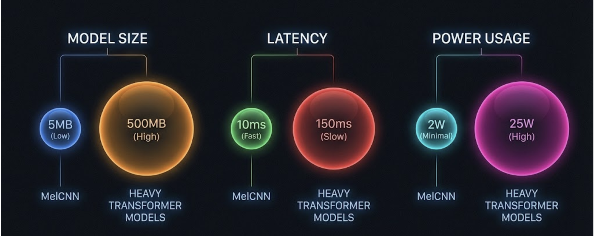
On edge devices, every millisecond and every megabyte matters. Audio models must run reliably on low-power CPUs, handle noisy real-world environments, and deliver consistent predictions without draining battery or storage. Traditional deep audio models—large transformers or multi-million-parameter networks—struggle here. They are powerful, but far too heavy for embedded hardware that also handles sensors, connectivity, and local analytics.

MelCNN is one of the few architectures that hits the “sweet spot”:

• Simple enough to run on edge CPUs without acceleration
• Accurate enough for real-world audio classification
• Compact enough to fit alongside other on-device ML workloads

For applications like dog-eating sound detection, barking segmentation, or anomaly detection—all relevant to Hoomanely’s on-device intelligence—MelCNN becomes a reliable backbone. It forms a fast, interpretable, resource-light approach to turning raw waveforms into actionable insights.

What Is MelCNN?

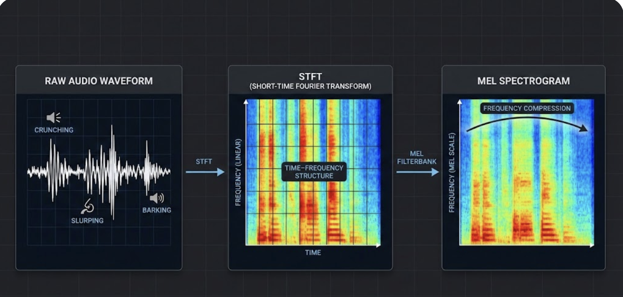
MelCNN is a convolutional neural network trained on Mel spectrograms. Instead of feeding raw audio to a heavy sequence model, MelCNN uses:

1. Short-Time Fourier Transform (STFT)
2. Mel filter banks to compress frequencies
3. 2D convolutional layers over time–frequency patches

This mirrors how image CNNs operate—except the “image” here is a compact time–frequency representation.

Why Mel Spectrograms?

• They shrink the audio: A few hundred Mel bins vs 16k raw samples per second.
• They preserve important structure: Harmonics, amplitude shifts, and texture.
• They are stable against noise: A big advantage for real outdoor audio.

The result: MelCNN learns patterns that correspond to acoustic events (like crunching, slurping, barking) without requiring heavy temporal modeling.

Why MelCNN Works Well for Audio Classification

MelCNN performs surprisingly well in constrained settings due to three practical strengths.

1. Parameter Efficiency

MelCNN’s convolution layers operate on a small 2D matrix, not long sequences. This keeps parameter counts low—often under 1–3M parameters, depending on depth.

2. Local Feature Learning

Audio events often have signatures like:

• Onset bursts (eating)
• Repeating rhythmic textures (chewing)
• Sharp transients (barks)
• Broadband noise (scratching)

CNNs capture these naturally through localized filters.

3. Robustness to Real‑World Noise

Random environmental noise affects spectrograms less dramatically than raw waveforms. Combined with convolutional smoothing, MelCNN builds resilience without expensive pre-processing.

4. Easy to Quantize & Optimize

MelCNN handles:

• INT8 quantization
• ONNX Runtime on CPU
• Pruning

with minimal accuracy loss. This makes it far easier to ship on embedded hardware than transformer-based models.

How MelCNN Works Internally

Here is the typical pipeline from microphone to output:

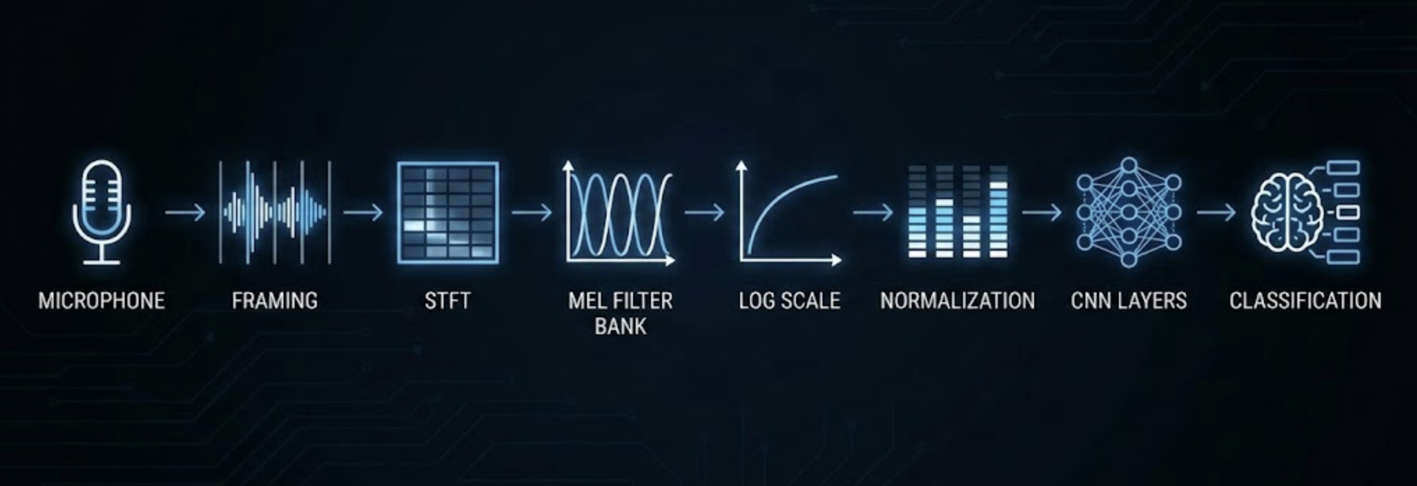
1. Raw waveform → 16kHz mono
2. Framing → split into 25ms windows
3. STFT → magnitude spectrogram
4. Mel filtering → compress to ~64–128 Mel bins
5. Log scaling → improve dynamic range
6. Normalize → per-speaker or global stats
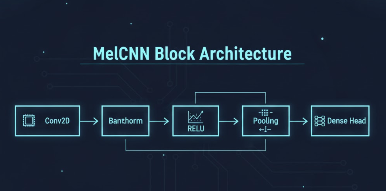
7. Conv layers → 3–5 blocks, ReLU, batch norm
8. Pooling → downsample time & frequency
9. Dense head → classification logits

The architecture is intentionally simple. The power lies in step 4: converting raw sound to the Mel domain where the patterns become visually structured.

Why MelCNN Shines on Edge Devices

Unlike transformer-based audio models, MelCNN is designed for resource-limited environments.

Small Model Size

Even a full model with 4 conv blocks often fits under 2–4 MB when quantized.

Low Compute Footprint

Spectrogram generation is lightweight and CNN inference is O(n·k) on a small input.

On Raspberry Pi-class hardware, MelCNN can reach 20–50 FPS depending on input length.

Predictable Latency

No recurrence. No attention layers. No dynamic shapes.

This ensures consistent timings—critical for real-time dog-eating detection.

Compatible with Multiple Runtimes

MelCNN runs efficiently on:

• ONNX Runtime
• TFLite
• PyTorch Mobile

That flexibility makes deployment reliable across different edge SKUs.

Use Cases

At Hoomanely, our edge devices process real-world audio directly inside pet homes. This audio is often:

• Mixed with ambient noise
• Captured at variable distances
• Subject to echoes, bowls, movement, and room acoustics

MelCNN helps us tackle problems such as:

1. Eating Sound Classification

Chewing, licking, and slurping all have strong Mel signatures. MelCNN can differentiate these even when background noise exists. This enables automated meal tracking.

2. Bark Detection

Barks have broadband structures that CNNs capture easily. MelCNN helps identify duration and intensity.

3. Activity & Anomaly Detection

Sudden changes in spectrogram structure can signal:

• Distress
• Reverse sneezing
• Cough-like events
• Unusual bowl interactions

MelCNN is fast enough to run continuously without overloading CPU or power.

Example Architecture (Simplified)

Input Mel Spectrogram (1 × 128 × 256)
│
├── Conv2D (32 filters, 3×3) → ReLU → BN
│
├── Conv2D (64 filters, 3×3) → ReLU → BN → MaxPool
│
├── Conv2D (128 filters, 3×3) → ReLU → BN
│
├── Global Average Pooling
│
└── Dense Layer → Softmax

Small changes in depth and channel sizes allow the model to scale up or down depending on hardware.

Strengths & Limitations

Strengths

• Very fast on CPU
• Low memory usage
• Works well with limited datasets
• Stable under noisy conditions
• Simple to deploy and maintain

Limitations

• Does not capture long-range temporal structure as deeply as transformers
• Needs careful preprocessing consistency
• Not ideal for multi-speaker or source-separation problems

For edge-level audio classification, however, MelCNN hits the ideal balance.

Key Takeaways

• MelCNN converts audio into a structured image-like form using Mel spectrograms.
• It is lightweight, robust, and extremely edge-friendly.
• Real-world tasks like eating detection or barking classification benefit from its speed and stability.
• At Hoomanely, MelCNN helps bring reliable on-device audio intelligence directly into pet homes.
• While not as expressive as transformer models, its efficiency makes it a strong backbone for real-time edge ML.