From 5.6% to 74%: What Ground Truth Did for Our Sleep Detector

In the first post in this series we described a rule-based sleep detector for our collar wearable: bucket the IMU stream into one-minute epochs, score each epoch by how much the acceleration is changing, and call a long enough run of quiet minutes a sleep bout. We ended that post by admitting we had one dog, one threshold picked by eye, and no ground truth. The plan was to go get some.

We did. Someone sat with a dog for eight days and wrote down, to the second, every time it settled and every time it got up. That gave us 31 observed rest sessions to check the algorithm against, all of them in daylight hours between late morning and mid-afternoon. The algorithm found zero of them.

This post is about what those eight days taught us, which turned out to have less to do with sleep than with timestamps.

Zero out of thirty-one

The scoring is deliberately generous. Take every minute inside an observed rest session, ask what the pipeline said about that minute, and count a session as detected if at least half its minutes came back as some flavour of rest. Under that rule, nothing. Twenty-one sessions had no data at all. Eight it confidently labelled active. Two were too short to score.

Measured only on the minutes where we actually had data, it recovered 5.6% of observed rest. On recall alone, a coin flip would have done better.

The one number that looked good was precision, at 100%. That is not the consolation it sounds like. It was 100% across seven minutes out of 463, which is what you get when a classifier almost never says yes.

Nothing in the feature's own output had flagged itself. It had been running for weeks producing numbers that were thin and uneven but never absurd, which is exactly why we wanted observer data rather than more dashboards.

The bug was in the clock, not the classifier

Roughly 62% of observed rest minutes had no data from the collar wearable at all. That part is not an algorithm problem, and we come back to it below. The interesting failure is in the minutes where data did arrive and the answer was still wrong.

To separate the two, we built a second view of the same days. Instead of trusting what the pipeline had computed, we went back to the raw batches and recomputed the movement feature per minute using the timestamps the collar wearable itself had assigned to each sample. That gives you a reference for what the accelerometer actually saw, independent of anything done to it after delivery.

The two views disagree spectacularly.

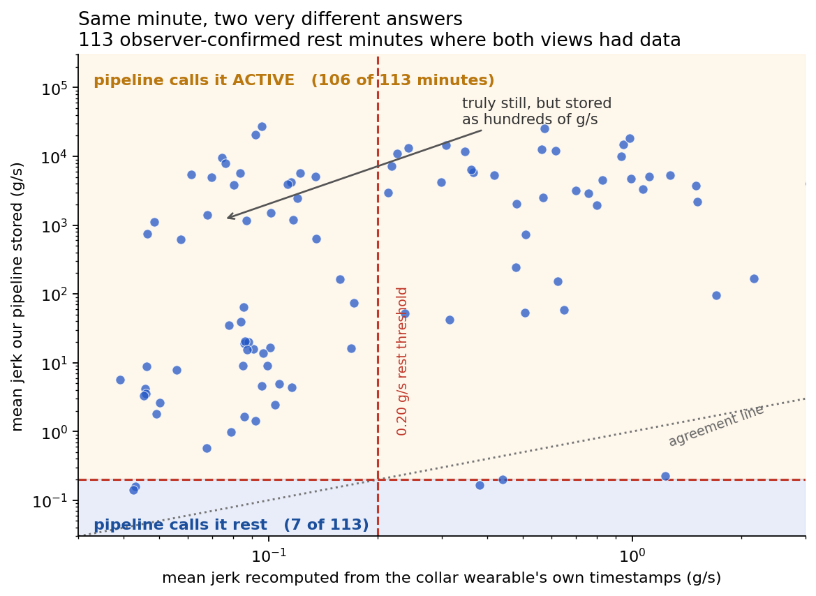
By the collar wearable's own timestamps, 54 of those 113 minutes are comfortably below the rest threshold. The pipeline called 7 of them rest. Same dog, same minute, same raw samples, and the stored number is often hundreds of times too big.

The cause is a design decision we described in the first post, and were rather pleased with at the time. The firmware's sample clock was boot relative, so it could not be used as wall time. Our fix was to anchor each batch of samples to the moment it was received, letting the firmware timestamps supply only the spacing within a batch. We wrote that this "keeps consecutive batches from drifting apart." It does. It also destroys the feature we care about.

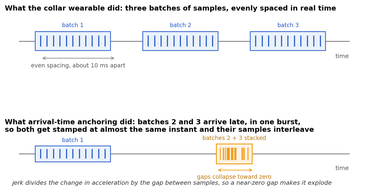
Our movement feature is a derivative. It divides the change in acceleration by the time between samples. Anchor two batches to the same instant and some of those gaps go to nearly zero, and dividing by nearly zero produces exactly the enormous numbers in that scatter plot. The dog was not moving. The arithmetic was.

Two smaller problems came out of the same investigation. The stream also carries a duplicate copy of some seconds of IMU, captured alongside audio events, and our exact-match duplicate filter sailed straight past copies whose timestamps differed by a millisecond. And some epochs had accumulated more samples than the collar wearable is physically capable of delivering in a minute, which should have been an obvious alarm and instead was silently classified as motion.

The signature of an intermittent fault

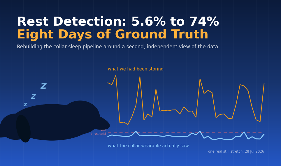
The most transferable thing we learned is what this class of failure looks like from the outside. The corruption was never a constant offset. Take one forty-minute stretch on 28 July where every raw measure says the dog did not move: the stored value ran from about 1 to 27,000 g/s. As an inflation factor that is twelve times at the mildest and 285,000 times at the worst, and it moves that fast between neighbouring minutes. At 12:05 the stored figure was roughly 225,000 times too high; one minute later it was 24 times too high. Fourteen of those forty minutes were inflated by less than a hundred times, and thirteen by more than ten thousand.

A constant offset would have been caught in a day, because every number would have been wrong in the same direction by the same amount and the threshold would obviously have needed moving. An intermittent fault is harder, because it produces output that jumps around minute to minute, and that is also a fair description of a real animal. The daily totals had the same shape. One day with overnight coverage reported about six hours of sleep; another reported none and called the dog active through most of the night. Both sit inside the range a real dog can produce, so neither pointed at the pipeline rather than the animal.

The answer to that is not closer reading of the same numbers, it is a second opinion, and building one is the most useful thing to come out of this work. We now have a reconstruction path that recomputes the movement feature directly from the timestamps the collar wearable assigned to each sample, independent of everything the delivery layer did to the batch afterwards. It runs over any archived day and produces a reference answer to set against whatever we stored at the time. That is what turned a vague sense that the signal was noisy into a specific, reproducible number, and it is the piece we did not have when we wrote the first post. Every figure in this post comes from running it.

One scope note while we are being precise. Every observed session is daytime, so nothing here validates those overnight figures either way: the six-hour night is not confirmed and the empty night is not confirmed. Doing that properly means watching a dog overnight, and it is on the list.

What we changed

Three of the four fixes are hygiene rather than cleverness.

The firmware now reports absolute timestamps, so the pipeline uses the device clock directly and only falls back to arrival-time anchoring for older batches that do not have it. Data from before that firmware change is effectively unusable for this feature, which we decided to accept rather than try to rescue. The duplicate audio-capture copies are excluded outright. Samples closer together than a few milliseconds get collapsed before the derivative is taken, and an epoch holding more samples than the stream can physically deliver is now marked unclassifiable instead of being called active. That last one matters more than it looks: the honest answer to corrupt input is to refuse it, not to guess.

Only the fourth change touches the classification rule itself, and we only found it because the first three had cleared the noise out of the way. With trustworthy timestamps, a chunk of observed rest minutes still failed the movement test. Looking at those minutes, the dog was clearly still, the acceleration barely varying, but the sample-to-sample change stayed elevated. That is what panting looks like through a collar. Steady, rhythmic, low amplitude, and not sleep-like at all by a derivative-based measure.

So an epoch can now qualify as rest two ways: the original movement test, or a stillness test on how much the acceleration magnitude varies across the minute. A panting dog lying down passes the second even when it fails the first.

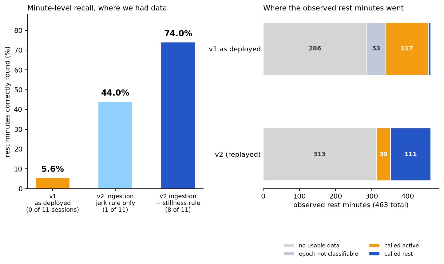
Recall on minutes with data goes from 5.6% to 44% on the timestamp fixes alone, then to 74% with the stillness test. Sessions detected go from 0 to 8 of the 11 that had usable data at all.

The numbers we are not going to dress up

Precision drops to 59% and the awake minutes we correctly leave alone fall to 50%. Read literally, we bought recall by becoming trigger happy.

We think the true figure is better than that, and we can say why without hand waving. Of the 77 minutes counted against us, 22 fall within two minutes of a session boundary, where a dog settling or stirring is genuinely ambiguous and the observer's stopwatch and the sensor will never agree to the minute. Of the 55 that are not near a boundary, 33 show an acceleration spread under 0.02 g, which is a dog that is not moving, while the sheet says awake. We cannot tell from the sensor alone which of those are the observer looking away and which are real, though at least one turned out to be a transcription slip that we found by following the sensor back to the sheet. A rule that fires on a dead-still dog is not obviously the thing that is wrong.

We are also not going to pretend these are unbiased numbers. The stillness threshold was tuned on the same eight days it is being scored against, so the honest version of this measurement is the one we take on days we have not seen yet. That is the next job.

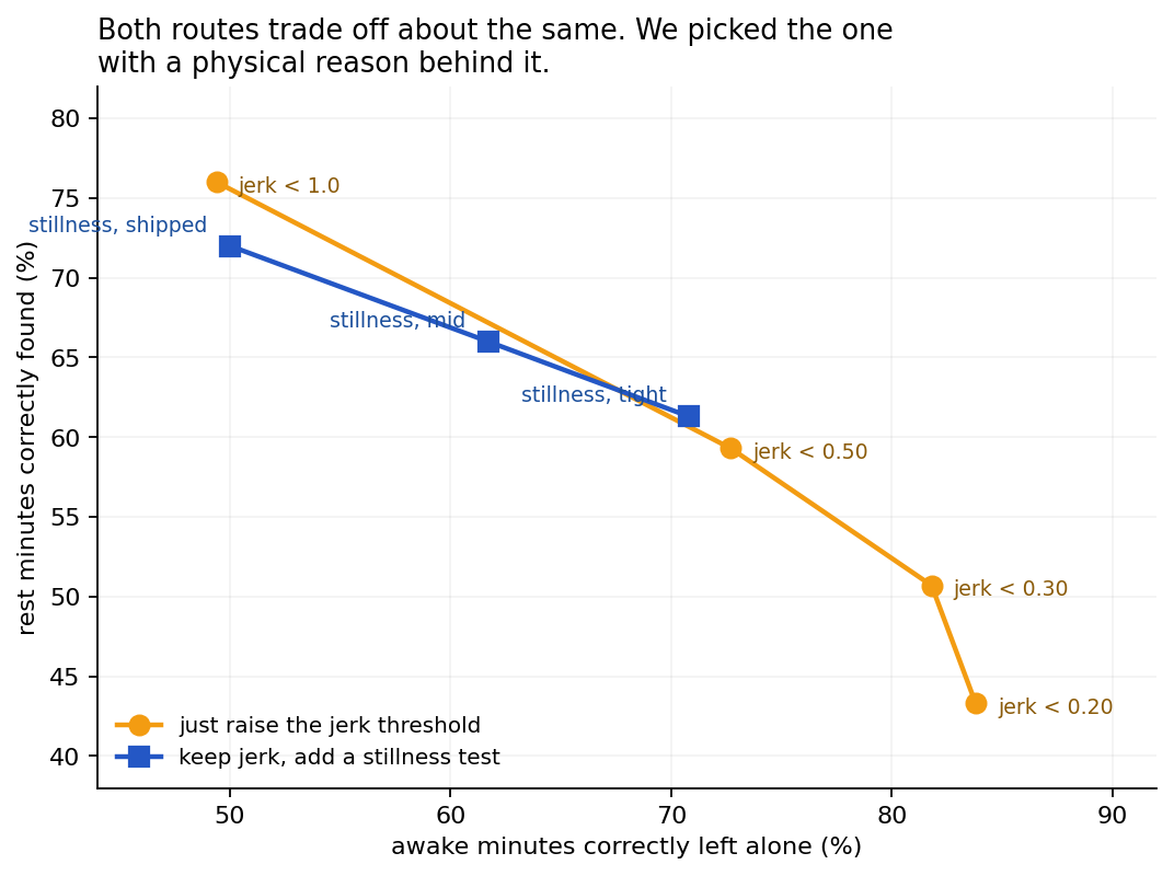
That last chart is the one that gave us pause. Sweeping the movement threshold upward buys almost the same recall as adding the stillness test. If you only look at the summary metrics, there is little to choose between them. We went with the stillness test anyway, because it fires for a reason we can name, and when it is wrong we will be able to see that a dog was still and panting rather than wondering why we tolerate more motion than we used to. Interpretability is not free performance, but it is what makes the next round of debugging possible.

The bigger problem is not the algorithm

Look again at the right panel above. In both versions, the largest block is minutes where no data ever arrived from the collar wearable, and it does not shrink, because no amount of classifier work can invent data that was never delivered. Eighteen of the twenty-one remaining missed sessions are pure gaps. There were hour-long stretches where our receiver sat there perfectly healthy, dutifully recording that it had received nothing, across four consecutive observed rest sessions.

That is now the top item, and it belongs to firmware and the wireless link rather than to signal processing. It is a less interesting problem than sleep staging and it is worth strictly more.

What we took away

The lesson we keep coming back to is not "test against ground truth," which everybody already knows. It is to pick a check for its sensitivity rather than its convenience. A single clean example and a couple of daily totals were the easiest things to look at, and this particular fault could pass all of them. Eight days of observer notes settled in one afternoon what output-watching could not, which is why the next threshold change gets measured against fresh observed days before it ships.

The other one is smaller and more practical. When a derivative-based feature goes wrong, suspect the denominator before the physics. We spent real time considering whether a collar on a dog's neck was simply a noisier place than we had assumed, and whether the threshold needed to be breed dependent, and whether panting was going to sink the whole approach. None of that was the problem. The problem was that we had quietly told the maths that two samples arrived at the same time.

The fixed version is deployed and stamps its events with a new algorithm version, so the next validation can tell cleanly which pipeline produced which day. We will report the fresh-data numbers when we have enough of them, including if they are worse than these.