Synchronizing Time Across Multiple SoMs: Building a Distributed Clock System

The Problem: When Time Doesn't Add Up

Picture this: You're debugging a critical issue in production. The logs show that a sensor event was processed before it was captured. Impossible? No-just unsynchronized clocks.

This was our reality when building distributed embedded systems. Our platforms rely on multiple Systems-on-Module (SoMs) working in concert, each handling different sensors and processing tasks. But without synchronized time, we were essentially flying blind.

Why Multiple SoMs? The Distributed Architecture Advantage

Modern embedded systems increasingly use multiple SoMs rather than a single monolithic computer. Consider our platforms - Everhub for edge computing and Everbowl for intelligent multi-sensor processing - both leverage this distributed architecture.

The Case for Distribution

Processing Distribution: When you have multiple high-bandwidth sensors (cameras, thermal imaging, audio streams), dedicating separate SoMs prevents resource contention. One SoM handles a subset of sensors while another processes different inputs simultaneously.

Thermal Management: High-performance processing generates heat. Distributing the computational load across multiple physical modules prevents thermal throttling and hotspots that plague single-board solutions under sustained load.

Isolation and Reliability: If one SoM encounters an issue or needs to reboot, the others continue operating. Critical communication functions remain available even if sensor processing temporarily fails.

Specialization: Each SoM can be optimized for its specific task—some configured for low-latency sensor capture, others for compute-intensive processing, and one dedicated to system coordination and external connectivity.

Scalability: Need to add more sensors? Integrate a new processing algorithm? Simply add or upgrade the relevant SoM without redesigning the entire system.

Parallel Processing: True hardware parallelism - multiple sensors being captured and processed simultaneously on different physical modules, not just different threads.

But this architectural elegance introduces a fundamental challenge: time synchronization.

The Challenge: When Every SoM Lives in Its Own Time

In a multi-SoM system, events happen across different modules constantly. Let's say you have a system with multiple SoMs where:

• SoM 1 handles certain sensors
• SoM 2 handles different sensors
• Master SoM coordinates communication

Real-world scenario:

• SoM 1 captures a sensor reading at its local timestamp
• SoM 2 processes data at its local timestamp
• Master SoM logs a system event at its local timestamp

Question: Which event actually happened first?

Without synchronized clocks, you simply cannot know. Each SoM's clock runs independently, and they drift apart over time.

What You Cannot Do Without Synchronized Time

1. Correlate Multi-Sensor Data

Modern systems fuse data from multiple sensors across different SoMs. Was one sensor's reading present when another sensor triggered? Without synchronized timestamps, correlation becomes guesswork.

2. Calculate True Latencies

How long did your processing pipeline take? If sensor capture happens on one SoM and processing completes on another, the calculated latency is meaningless if the clocks disagree.

3. Reconstruct Event Sequences

During debugging or incident analysis, you need to reconstruct what happened. But if logs from different SoMs have inconsistent timestamps, you might see effects appearing before causes—making root cause analysis impossible.

4. Perform Accurate Sensor Fusion

Sensor fusion algorithms depend on temporal alignment. If data from different SoMs has misaligned timestamps due to clock drift, fusion algorithms produce incorrect results or miss detections entirely.

5. Meet System Requirements

Many applications have hard timing requirements:

• Real-time systems need provable maximum latencies
• Safety-critical systems require timing certification
• Data logging must have consistent, auditable timestamps
• Synchronization with external systems demands a common time reference

Example: The Multi-Sensor Detection Problem

Consider a system detecting events using sensors distributed across SoMs:

1. Sensor on SoM 1 detects signature
2. Sensor on SoM 1 captures additional data
3. Sensor on SoM 2 picks up related signal
4. Sensor on SoM 1 confirms reading

Question: Are these sensors detecting the same event or different events?

For accurate sensor fusion and event correlation, you need to know:

• Are these from the same object/event or different occurrences?
• What's the temporal correlation?
• Which sensor detected it first?
• What's the propagation delay between sensors?

With unsynchronized clocks, even if all sensors detect the same event simultaneously, the timestamps could differ significantly—making fusion algorithms produce incorrect results.

The Physics of the Problem: Clock Drift is Inevitable

Every SoM has its own crystal oscillator driving its system clock. These crystals are imperfect physical devices, not perfect timekeepers.

Why Crystals Drift

Environmental Factors:

• Temperature: Crystals change frequency with temperature. A temperature change causes the crystal to oscillate faster or slower, changing the rate at which the clock ticks.
• Supply voltage fluctuations: The oscillator's frequency depends on stable power. Voltage variations cause frequency variations.
• Mechanical stress: Physical vibration affects the crystal's resonance frequency. In moving platforms or environments with machinery, this is significant.
• Electromagnetic interference: External radio frequency signals can modulate the oscillator frequency.

Manufacturing Variability:

• Tolerance: Even brand new crystals have inherent frequency tolerance from their nominal specification. No crystal oscillates at exactly its rated frequency.
• Aging: Crystal frequency drifts over months and years as the material properties change.
• Unit-to-unit variation: No two crystals behave identically, even from the same manufacturing batch.

Real-World Impact

Even with high-quality crystals, clocks drift apart over time:

• Short term (seconds to minutes): Small but measurable drift begins
• Medium term (hours): Drift accumulates noticeably
• Long term (days): Clocks can be significantly out of sync

Practical implications:

Two SoMs powered on at the same moment will show different clock readings within minutes. The difference grows continuously. Temperature changes accelerate drift.

Consider this: If one SoM is processing heavy computations and runs warmer, while another SoM handles lighter loads and stays cooler, their clock drift rates will be different. The warmer SoM's crystal may drift faster than the cooler one's.

Why One-Time Calibration Doesn't Work

You might think: "Let's just measure the clock offset once at startup and correct for it!"

Problem: Drift accumulates continuously.

Even if you perfectly calibrate clocks at startup:

• Temperature changes during operation cause frequency drift
• The SoM that was cool at startup warms up and its clock frequency changes
• Supply voltage variations cause additional drift
• Clock drift is not constant—it changes with environmental conditions

If you calibrate at room temperature startup, but then the system heats up during operation, the calibration becomes invalid within minutes.

You need continuous, active synchronization.

The Solution: A Master Clock and Synchronization Protocol

Our solution designates one SoM as the master clock (the time authority) and implements a synchronization protocol that continuously corrects the other SoMs' clocks.

Architecture Overview

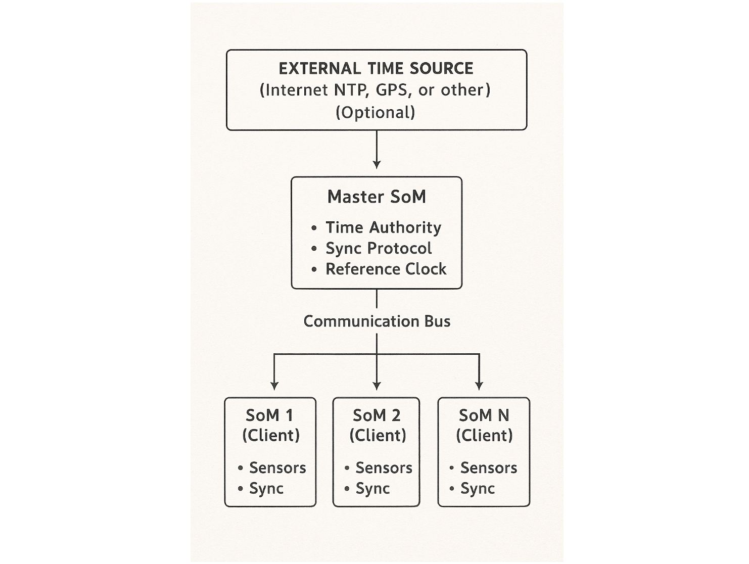
Design Principles

Master SoM Selection: Choose the SoM that:

• Has external connectivity (useful for synchronizing to absolute time sources like NTP or GPS, though optional)
• Has a stable thermal environment (SoMs with lower processing loads tend to have less thermal variation)
• Has reliable power supply
• Plays a central coordination role in the system

Client SoMs: All other SoMs become time clients. They periodically synchronize their local clocks to the master's reference time.

Communication: The SoMs communicate over whatever bus connects them—CAN, Ethernet, SPI, or any other protocol. The synchronization algorithm adapts to the communication medium's characteristics.

Why this works: Instead of having each SoM try to keep perfect time independently (impossible with crystal drift), we establish one reference clock and continuously measure and correct the differences between that reference and each client's local clock.

The Core Algorithm: Measuring and Correcting Clock Offset

The synchronization process needs to answer one fundamental question: "How different is my clock from the master's clock?"

This is trickier than it sounds because the very act of asking the question takes time—messages don't travel instantaneously between SoMs.

Step 1: Clock Offset Measurement

The Protocol (Cristian's Algorithm):

When a client SoM wants to synchronize:

1. Client sends sync request to master, recording its local time as t0
2. Master receives request, timestamps it as t1 using the master's clock
3. Master sends response containing the timestamp t1
4. Client receives response, recording its local time as t3

Now the client has three timestamps: t0 and t3 from its own clock, and t1 from the master's clock.

The Calculation:

Round-Trip Time (RTT) = t3 - t0
  (This is how long it took for the request to go to master and response to return)

Estimated One-Way Delay = RTT / 2
  (Assuming symmetric delay—message takes similar time in both directions)

Clock Offset = t1 - (t0 + One-Way Delay)
             = t1 - (t0 + RTT/2)

Error Bound = RTT / 2
  (Our uncertainty in the measurement)

Why this works:

If we assume the message takes roughly the same time traveling from client to master as from master to client (symmetric delay), then when the master timestamped the request at t1, the client's clock should have read t0 + RTT/2.

The difference between what the master's clock said (t1) and what the client's clock should have said (t0 + RTT/2) reveals the clock offset between them.

Visual Example:

Imagine the client's clock reads 1000.000 ms when it sends the request. The response returns when the client's clock reads 1000.003 ms. The RTT is 3 microseconds.

If the message traveled symmetrically, it took 1.5 microseconds each way. So when the master received the request and timestamped it, the client's clock should have read 1000.0015 ms.

But suppose the master's timestamp says 2000.010 ms. This means the client's clock is behind the master's clock by approximately 2000.010 - 1000.0015 = 1000.0085 milliseconds.

Now the client knows: "My clock is about 1000 ms behind the master."

The Key Insight: We've measured the clock offset despite the communication delay by using the round-trip time to estimate when the master's timestamp corresponds to in the client's time frame.

Step 2: Handling Communication Variability

Not all sync measurements are equally reliable. Communication delay varies due to:

• Message queuing in buffers (other traffic delays our sync messages)
• CPU scheduling delays (the receiving SoM might be busy with other tasks)
• Interrupt latency (delay before the timestamp is actually captured)
• Bus contention (multiple devices trying to communicate simultaneously)

The Problem: If a sync request gets delayed in a queue for 5 milliseconds, but we assume symmetric delay, our offset calculation will be wrong by about 2.5 milliseconds.

Solution: Weight measurements by their quality.

We track the minimum observed RTT over recent measurements. This represents the "best case" communication delay—when the path is clear with no queuing or contention.

When a new measurement arrives:

• If its RTT is close to the minimum, it's a high-quality measurement with little delay variation
• If its RTT is much higher, it likely suffered from queuing or contention, making it less reliable

We give higher weight to measurements with low RTT and lower weight (or completely discard) measurements with suspiciously high RTT.

Example: If our minimum observed RTT is 500 microseconds, and a new measurement has RTT of 550 microseconds, we trust it highly. But if a measurement has RTT of 5000 microseconds, we know something delayed it—probably queuing—and we either discard it or weight it very lightly.

This strategy filters out measurements corrupted by communication delays, keeping only the clean, reliable measurements.

Step 3: Correcting Two Types of Error

Simple offset correction isn't enough. Clock drift has two independent components that need separate treatment:

1. Phase Error: The current clock offset (e.g., "my clock currently reads 5ms behind master")
2. Frequency Error: The rate of drift (e.g., "my clock gains 50 microseconds per second relative to master")

Why both matter:

If you only correct phase (just adding 5ms to fix the current offset), the underlying frequency error means the clocks immediately start drifting apart again. Within seconds, you're out of sync again.

If you only correct frequency (adjusting how fast the clock ticks), you fix the drift rate, but the initial offset remains. You still have the 5ms error, even though it's not getting worse.

You need to correct both simultaneously.

The Challenge: With a single correction mechanism, frequency adjustments interfere with phase corrections. When you adjust the clock rate to fix frequency, it looks like a phase error. When you adjust the offset to fix phase, it looks like a frequency error. The system fights itself and never converges stably.

The Solution: Two-stage correction process with independent controls.

┌──────────────┐     ┌───────────────┐     ┌───────────────┐
│   Master     │────►│   Virtual     │────►│   Virtual     │────►Synchronized
│   Reference  │     │   Clock #1    │     │   Clock #2    │     Time
│   Clock      │     │               │     │               │
└──────────────┘     └───────┬───────┘     └───────┬───────┘
                             │                     │
                      ┌──────▼─────────┐   ┌──────▼─────────┐
                      │  Frequency     │   │  Phase         │
                      │  Correction    │   │  Correction    │
                      │  (slow loop)   │   │  (fast loop)   │
                      └────────────────┘   └────────────────┘

Stage 1 - Frequency Correction (slow, long-term):

This stage observes how the phase offset changes over time. If your clock is consistently gaining 50 microseconds per second relative to the master, this indicates a frequency error.

The frequency correction adjusts a virtual clock's tick rate. If the local crystal runs slightly fast, we slow down the virtual clock proportionally. If it runs slow, we speed up the virtual clock.

Measurements are taken over long intervals (many seconds) because frequency is a rate-of-change measurement. You need to observe the accumulated drift over time to accurately measure the frequency error. This long measurement window also filters out short-term noise and communication jitter.

Stage 2 - Phase Correction (fast, short-term):

This stage measures the instantaneous phase offset between the (now frequency-corrected) virtual clock and the master.

It directly adjusts the clock phase to eliminate the current offset. If there's still a 2ms offset after frequency correction, the phase correction adds 2ms.

Measurements are taken frequently (every second or few seconds) to quickly eliminate transient errors and respond to sudden changes.

Why two stages work:

The frequency correction provides a stable foundation—a clock ticking at approximately the right rate. The phase correction makes fine adjustments on top of that stable base. They don't interfere because they operate on different time scales and different aspects of the clock (rate vs. offset).

This approach is called a "phase-locked loop" (PLL), a well-established control theory technique. The two-stage design gives us two "degrees of freedom" allowing the system to independently control both frequency and phase, achieving rapid and stable convergence.

Step 4: Tracking Accuracy Over Time

Between synchronization measurements, we don't know exactly how accurate our clock is. The error grows as time passes since the last sync.

Every timestamp comes with an error estimate:

Current_Error = Last_Measurement_Error + (Time_Since_Last_Sync × Residual_Uncertainty)

Components:

Last_Measurement_Error: This comes from the RTT of the last sync measurement. If RTT was 1000 microseconds, our measurement error is approximately 500 microseconds (RTT/2). This is the inherent uncertainty in that measurement.

Residual_Uncertainty: Even after frequency correction, there's still some unmeasured drift. The frequency correction isn't perfect—temperature might be changing, the crystal might be aging. We estimate this residual drift rate (typically a few parts per million).

Time_Since_Last_Sync: The longer since our last sync measurement, the more uncertainty accumulates due to residual drift.

Example:

Last sync measurement had RTT of 1000 microseconds, giving measurement error of 500 microseconds. Our residual frequency uncertainty is 10 PPM (parts per million), meaning 10 microseconds per second. If 5 seconds have passed since the last sync:

Current_Error = 500 µs + (5 seconds × 10 µs/second)
              = 500 µs + 50 µs
              = 550 µs

Our current timestamp has an estimated error bound of 550 microseconds.

Out-of-Sync Detection:

If Current_Error exceeds your accuracy requirement (say, 1000 microseconds), the system enters out-of-sync state:

• Stops providing timestamps (prevents delivering bad data)
• Logs a warning for system diagnostics
• Attempts more frequent synchronization to recover
• Resumes normal operation once error drops below threshold

Critical design principle: Rather than delivering timestamps with unknown accuracy, we fail explicitly and loudly when we cannot meet requirements. Silent failures with bad timestamps corrupt data and cause subtle bugs. Loud failures are debuggable.

Implementation Philosophy: The Transform Function Approach

We deliberately do not adjust the operating system's clock. Instead, we maintain a mathematical transform function that converts local monotonic time to synchronized time.

Why Not Adjust the System Clock?

Privilege Requirements: Adjusting system clocks typically requires administrator or root privileges. Applications running as regular users can't modify the system clock. This would force our synchronization service to run with elevated privileges, violating the principle of least privilege.

Software Conflicts: If other time services are running (like NTP daemon, systemd-timesyncd, or chronyd), they'll fight with our service for control of the system clock. They'll undo our adjustments, and we'll undo theirs, creating oscillations and instability.

Application Compatibility: Some applications expect monotonic time—time that only goes forward, never backward. If we adjust the system clock backward to correct an offset, applications might malfunction. Databases, loggers, and many other programs depend on monotonic time.

Flexibility: By not touching the system clock, different processes can theoretically synchronize to different time references if needed (useful for testing or multi-master scenarios).

How the Transform Function Works

Instead of changing the underlying hardware clock, we mathematically transform its readings.

The concept: We maintain parameters describing the relationship between local time and synchronized time:

• Phase offset: A constant offset to add (e.g., "add 1000 milliseconds to local time")
• Frequency multiplier: A scaling factor for elapsed time (e.g., "local clock runs 1.0001× too fast, so multiply elapsed time by 0.9999")

When application code requests the current synchronized timestamp:

1. Read the local monotonic clock (the hardware clock that always advances forward)
2. Calculate how much time has elapsed since our reference point
3. Apply the frequency correction to that elapsed time (scale it by the multiplier)
4. Add the phase offset
5. Return the result as the synchronized timestamp

Example:

Suppose at some reference moment, local clock read 1000.000 seconds and we determined that corresponded to 5000.000 seconds in master time. Now, local clock reads 1005.000 seconds—5 seconds have elapsed locally.

If our frequency correction is 0.9999 (local clock runs slightly fast), corrected elapsed time is 5.000 × 0.9999 = 4.9995 seconds.

If our phase offset is +0.002 seconds, synchronized time is 5000.000 + 4.9995 + 0.002 = 5004.9995 seconds.

We've converted local time 1005.000 into synchronized time 5004.9995 without ever touching the system clock.

Benefits:

• Works as an unprivileged user process
• No interference with system clock or other time services
• Clean, mathematical transformation that's easy to test and validate
• Robust against system clock adjustments by other software

Updating the Transform

As sync measurements arrive, we update the transform parameters using the two-stage correction process described earlier.

The frequency discipline updates the frequency multiplier based on long-term drift observations. The phase discipline updates the phase offset based on short-term measurements.

Both updates use "gains" (weighting factors) that control how aggressively we respond to measurements. Too aggressive causes oscillation and instability. Too conservative causes slow convergence. The gains are tuned through testing to achieve rapid convergence with stability.

Practical Considerations

Thread Safety

The synchronization service must handle concurrent access from multiple threads safely.

Multiple application threads might request timestamps simultaneously while a background thread is updating the transform parameters based on new sync measurements. Without proper synchronization, race conditions could cause corrupted timestamps or crashes.

We use mutexes (mutual exclusion locks) to ensure atomic operations:

• Reading the transform parameters requires locking
• Updating the transform parameters requires locking
• The sync status flag uses atomic operations for lock-free checking

The implementation minimizes lock contention by checking sync status with a fast atomic read before attempting the slower locked read of transform parameters.

API Design

Simple API: For most applications, provide a straightforward interface:

• get_timestamp(): Returns current synchronized timestamp or error if out of sync
• is_synchronized(): Checks if the clock is currently synchronized

Advanced API: For applications with strict timing requirements, provide detailed information:

• get_timestamp_with_error(): Returns timestamp plus error bound and sync status
• Applications can decide whether the current accuracy is sufficient for their needs

Example use case: A sensor fusion algorithm might require sub-millisecond accuracy. It calls get_timestamp_with_error(), checks if error bound is below 1000 microseconds, and only proceeds with high-accuracy fusion if the requirement is met. Otherwise, it falls back to a degraded mode or skips that fusion cycle.

Configuration

Each SoM has a configuration file specifying its role and parameters:

Master configuration:

• Role: master
• Whether to sync to external time source (NTP/GPS)
• External time source address if enabled

Client configuration:

• Role: client
• Master SoM identifier/address
• Sync interval (how often to request sync)
• Maximum acceptable error bound
• Various tuning parameters (gains, RTT thresholds, etc.)

Adaptive synchronization:

Rather than syncing at a fixed rate, intelligent implementations adapt:

• Start with frequent syncs (every few hundred milliseconds) during initial lock acquisition
• Gradually increase interval (up to several seconds) once stably synchronized
• Return to frequent syncs if error bound starts growing
• Balance accuracy requirements against communication and CPU overhead

Master SoM Implementation

The master SoM runs a simple service that responds to sync requests:

When a sync request arrives from a client:

1. Read the master's current time from its local clock
2. Send that timestamp back to the requesting client
3. Done

The master doesn't need to track clients or maintain per-client state. Each sync request is independent.

Optionally, the master can synchronize its own clock to an external absolute time source (NTP server over the internet, GPS receiver, etc.). This isn't required for relative synchronization between SoMs, but provides absolute UTC time if needed.

Communication Abstraction

The sync protocol works over various communication media—CAN bus, Ethernet UDP, SPI, shared memory, etc. The core algorithm (measure RTT, calculate offset, update transform) remains the same.

An abstraction layer handles media-specific details:

• How to send sync requests
• How to receive sync responses
• How to encode/decode timestamps in messages
• Media-specific timing characteristics

This allows the same synchronization code to work across different hardware platforms and communication protocols by simply swapping the communication backend.

Performance Expectations

The achievable accuracy depends on several factors:

Communication Characteristics:

• Latency: Lower latency enables better accuracy. Fast communication (microseconds) supports sub-millisecond sync.
• Jitter: Consistent delay is more important than low delay. Highly variable delay degrades accuracy.
• Reliability: Dropped messages require retransmission, degrading sync frequency.

System Characteristics:

• Temperature stability: Thermal transients cause frequency drift, requiring more frequent sync.
• Processing load: Heavy CPU load can delay message handling, increasing jitter.
• Clock quality: Better crystals (TCXO vs. standard crystal) have less drift, easier to synchronize.

Typical Results:

With well-designed systems (low-latency communication, moderate thermal stability, reasonable processing load), sub-millisecond synchronization is routinely achievable. Many deployments achieve accuracy in the hundreds of microseconds.

With challenging conditions (high-latency or jittery communication, severe thermal transients, heavy processing load), accuracy degrades but typically remains within a few milliseconds.

The Key Characteristic: The system continuously measures and reports its own accuracy. You always know how accurate your timestamps are. The system degrades gracefully—accuracy gets worse under stress, but predictably and measurably. When accuracy becomes unacceptable, the system detects this and reports it rather than silently delivering bad data.

Validation and Testing

Stress Testing

Introduce challenging conditions deliberately:

• Network stress: Generate burst traffic to increase communication delays
• Thermal stress: Use thermal chambers or heat guns to create temperature transients
• Processing load: Run CPU-intensive tasks to create scheduling delays
• Long duration: Run continuously for days or weeks to observe long-term behavior

This reveals how the system behaves under real-world stress and validates graceful degradation. Good synchronization systems maintain accuracy even under stress, and when they can't, they detect and report the problem rather than silently failing.

Common Pitfalls to Avoid

Don't assume one-time calibration suffices: New developers often think "just measure the offset at startup." This fails within minutes as thermal drift accumulates. You need continuous, active synchronization throughout system lifetime.

Don't ignore communication variability: Treating all measurements equally degrades accuracy. Some measurements are corrupted by delays. Weight or discard poor measurements.

Don't silently deliver bad timestamps: It's tempting to always return something. But returning inaccurate timestamps without warning corrupts data and causes mysterious bugs. Better to fail explicitly.

Don't forget thermal management: Clock drift is largely temperature-driven. Systems that don't manage thermal environment see worse synchronization performance. Consider thermal design early.

Don't skip validation: It's easy to implement sync code that seems to work but has subtle bugs. Always validate with hardware ground truth and statistical analysis.

Conclusion

Synchronizing time across multiple SoMs is fundamental to building reliable distributed embedded systems. Without it, you cannot:

• Correlate multi-sensor data accurately
• Measure true system latencies
• Debug timing-related issues
• Perform accurate sensor fusion
• Meet safety or compliance requirements

The solution we've described combines several key elements:

• One SoM designated as master clock (time authority)
• Cristian's algorithm for measuring clock offset despite communication delay
• Two-stage phase-locked loops for independently correcting frequency and phase
• Transform function approach avoiding system clock modification
• Continuous accuracy tracking with explicit error bounds
• Graceful degradation and loud failure when requirements can't be met

With proper implementation, sub-millisecond time synchronization is achievable across all SoMs using commodity hardware with no specialized timing equipment. This enables sophisticated applications - from industrial automation to intelligent sensor systems—to operate reliably with precise, consistent timing across all distributed components.

The investment in time synchronization infrastructure pays dividends throughout the system lifecycle: faster debugging (timestamps actually mean something), more reliable operation (sensor fusion works correctly), and confidence that your distributed system's view of time is consistent and accurate.

Building this infrastructure takes effort upfront, but the alternative - dealing with unsynchronized clocks—causes endless debugging pain and unreliable systems. Get time synchronization right from the start.

Key Takeaway: Don't assume your SoMs' clocks agree. They don't, and they never will without active synchronization. Build synchronization in from the beginning, track accuracy explicitly, and fail loudly when precision degrades. Your future debugging self will thank you.